How Risky is a Correlated Hedge?

When investors think about hedging, they often look for assets or strategies that move in opposite directions. A friend of mine once said:¹

I’m buying some Exxon stock but am worried that something will affect the whole oil industry, so I’m also going to short Chevron.

They’re almost 90% correlated, so that should eliminate most of the risk.

Unfortunately, no. This is a fundamental misunderstanding of correlation. Even in an ideal scenario, a 90% correlation can only produce about a 50% reduction in risk.

While correlation measures how two assets move together, it doesn’t mean their future moves will cancel each other out.

Exxon vs. Chevron historical analysis

#

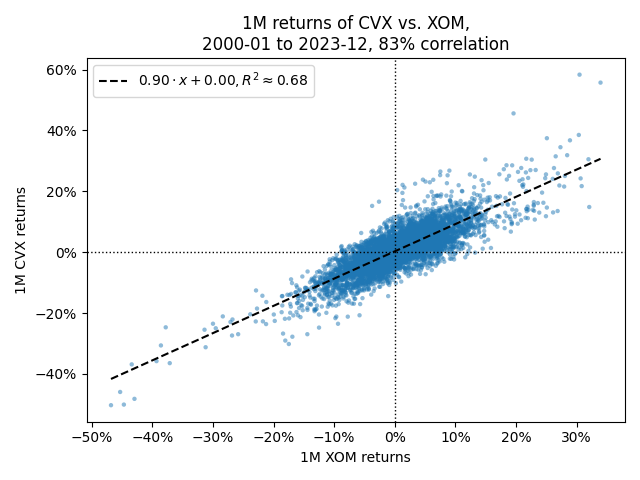
First, let’s plot the historical returns of Exxon (XOM) and Chevron (CVX) from the last few decades.

You can immediately see that while the stocks are highly correlated, this doesn’t mean their returns move perfectly together. If they did, the scatterplot would form a much tighter and more linear pattern.

Indeed, if we plot a histogram of historical returns before and after adding the Chevron hedge, you’ll find that the risk only drops by about 1/3rd! Why is that?

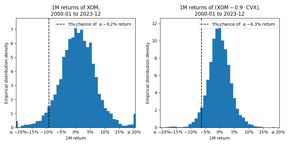
Roughly speaking, adding a hedge introduces some new risk of its own, so the correlation needs to be extremely high to counteract the combined volatility. Otherwise, there is still significant risk from idiosyncratic effects.²

Simplified statistical analysis

#

To better understand this hedge, let’s assume that the returns of both positions are normally distributed.

$$ X \sim \mathcal{N}\left(0, \sigma_X^2\right), \quad Y \sim \mathcal{N}\left(0, \sigma_Y^2\right), \quad \mathrm{Corr}(X, Y) = \rho $$

From this, we can derive the variance of returns for the hedged strategy. $$ \implies \mathrm{Var}(X-Y) = \sigma_X^2 + \sigma_Y^2 - 2 \cdot \rho \cdot \sigma_X \cdot \sigma_Y $$

So, if we’re hedging in such a way that both positions have the same volatility, \( \sigma_X = \sigma_Y \), we have

$$ \begin{aligned} \sigma_{X-Y} &= \sqrt{\sigma_X^2 + \sigma_X^2 - 2 \cdot \rho \cdot \sigma_X^2}\\ &= \sigma_X \sqrt{2\left(1-\rho\right)} \end{aligned} $$

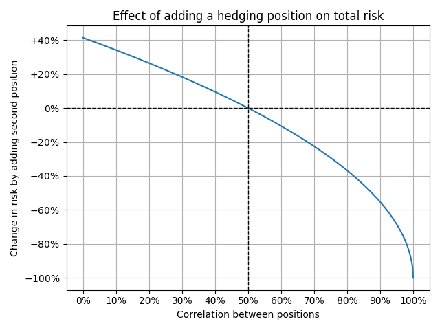
At the extremes,

• A 0% correlation increases the risk about 41% to \( \sqrt{2} \), which is exactly what you would expect from adding two independent standard normal variables together.
• A 50% correlation keeps the risk unchanged \(\left( \sqrt{2\cdot(1-0.5)} = 1 \right)\). I.e., it only cancels out the additional risk from the hedge itself.
• A 100% correlation decreases the risk to zero since it represents a perfect hedge.

In our earlier Exxon vs. Chevron example, with an ~83% correlation, we would expect a risk reduction of \( \sqrt{2 \cdot (1-83\%)} - 1\approx 42\% \) rather than the ~1/3rd we observed. Indeed, a few more real-world factors are at play here.

Other factors

#

• Stocks do not perfectly follow correlated normal random variables. Discrepancies from this behavior will typically reduce the risk reduction compared to an idealized analysis.
• Stock returns are often fatter-tailed than a normal distribution. This means that the risk tends to be worse than a normal analysis would suggest,³ particularly during extreme market events. A tail event in one asset could easily undermine any historical correlations you’ve observed.
• As usual, past performance is not indicative of future results. Relying on historical analysis, especially from long time frames, means accepting the risk that these trends may change in the future.

Ultimately, hedging with correlated assets can be useful in risk management, but it’s more complex than just seeing a high correlation and assuming that most of your risk can be hedged away.

See also and references

#

• General overviews of hedging can be found on Investopedia and Wikipedia.
• A more specific discussion of what I’m calling a “correlated hedge” is available in Investopedia’s article on “Cross Hedging”.
• The risk of a single asset not following the broader market is often referred to as Idiosyncratic Risk, Specific Risk, or Unsystematic Risk.
• Some fatter-tailed distributions that better approximate financial markets than a normal distribution include Stable Distributions and t-Distributions.
• A few warnings from a Reddit thread about a user who wanted to perform a similar hedge with options.