Converting Between Fat-Tailed Distributions

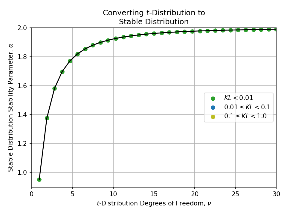
If I say “this data looks like a stable distribution with \( \alpha \approx 1.8 \)” and you feel it’s “more like a \(t\)-distribution with around 4 degrees of freedom”, are we basically saying the same thing?

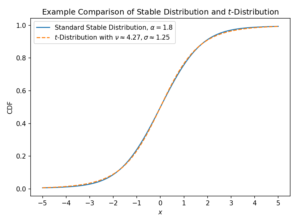
This is a pretty common thing to run into when modelling empirical data, so I wanted to generate some rules of thumb to “translate between the languages of various distributions”, so to speak.

Unfortunately, simple series expansions and asymptotic analyses are not very enlightening, so we need to do something a bit more complicated.¹

Methodology

#

Assume we have a distribution \(X\) with parameter \(\alpha\) that controls how heavy the tails are.

We want to find the “tailedness” parameter \(\beta\) from a different family \(Y\) that best approximates it.

To do this, we’ll be minimizing the Kullback-Leibler (KL) divergence between the two distributions. $$ \beta^{*} = \underset{\beta}{\text{arg min}}\ \underset{\sigma}{\text{min}} \left[\int_{-\infty}^{\infty} f_X(x; \alpha) \cdot \log\left(\frac{f_X(x; \alpha)}{f_Y(x; \beta, \sigma)}\right) \text{d}x\right] $$

This is equivalent to a maximum likelihood estimation fit of model distribution \(Y\) onto true distribution \(X\).

Note:

• The underlying optimization is multidimensional since these distributions have different inherent scales.²

  For example, a standard stable distribution with \(\alpha = 2\) is actually a normal distribution with standard deviation \(\sigma = \sqrt{2}\).

• This is not symmetric due to the asymmetry of KL divergence and maximum likelihood fitting.

  For similar distributions, converting in one direction \((X \to Y)\) will be close to the other direction \((Y \to X)\), but they are not the same in general.

Distributions of interest

#

Here, I am interested in all common³ symmetric distributions that have a single parameter controlling the heaviness of the tails. When necessary, skewness parameters are set to zero.

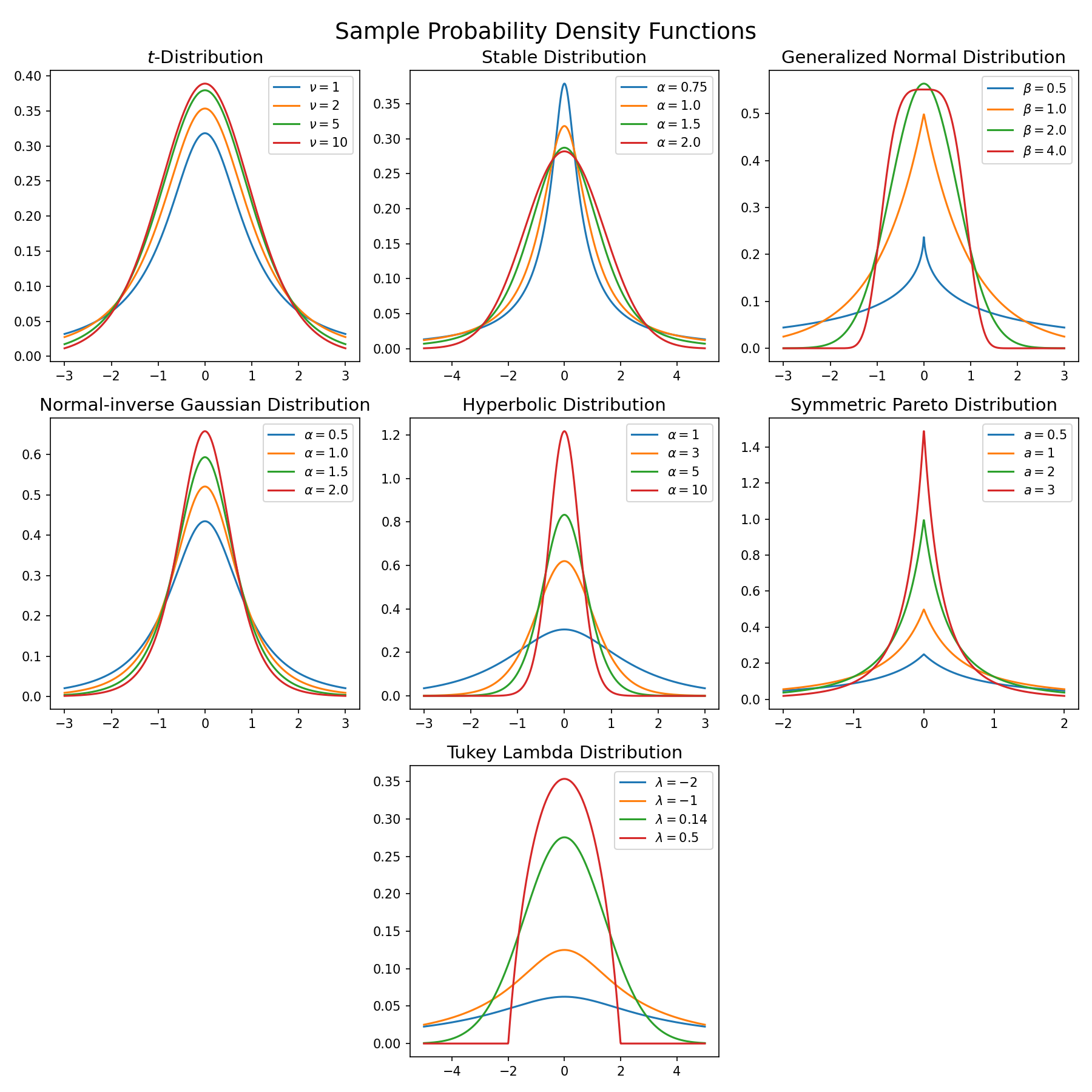
In all cases, decreasing the tail parameter yields fatter tails.

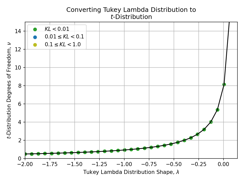
1. Student’s t-distribution
   • Tails are controlled by \(\nu > 0\) “degrees of freedom”
   • \(\nu = 1\) is a Cauchy distribution and \(\nu \to \infty\) is a normal distribution
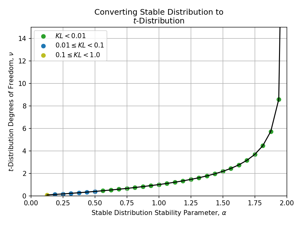
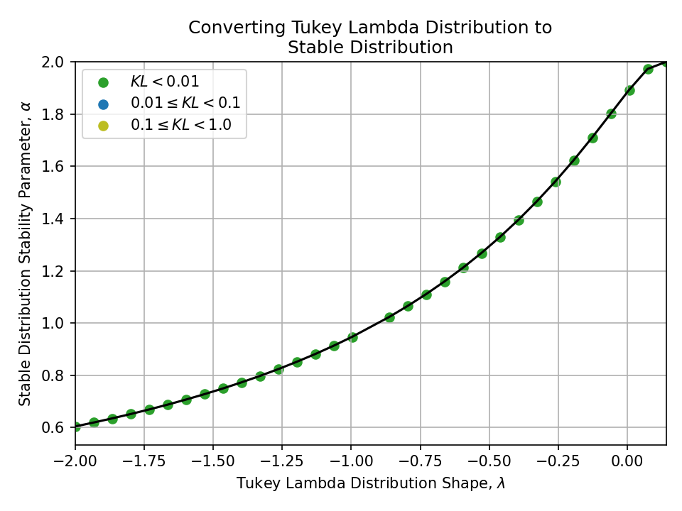
2. Lévy alpha stable distribution
   • Tails are controlled by stability parameter \(\alpha \in (0, 2]\)
   • \(\alpha = 1\) is a Cauchy distribution and \(\alpha = 2\) is a normal distribution
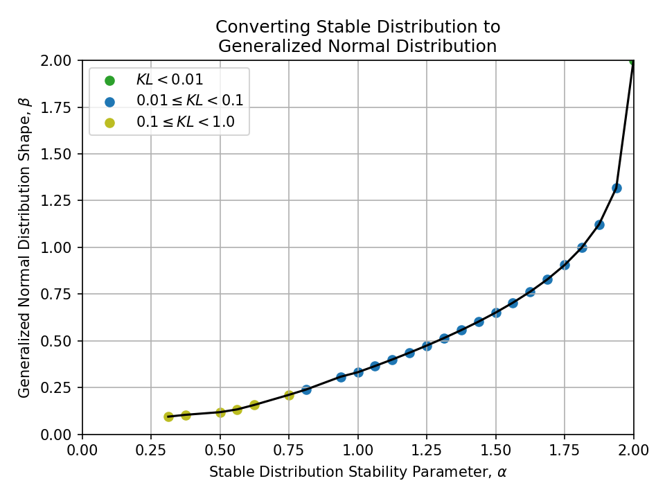
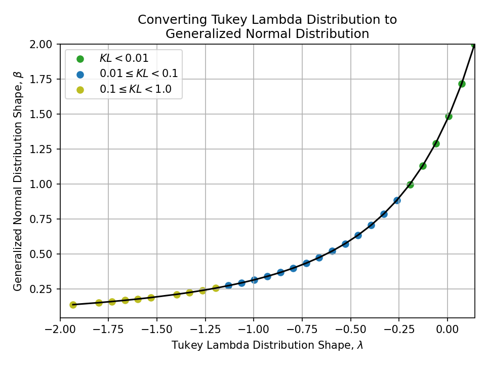
3. Generalized normal distribution
   • Tails are controlled by shape \(\beta \in \mathbb{R}\)
   • \(\beta = 1\) is a Laplace distribution, \(\beta = 2\) is a normal distribution, and \(\beta \to \infty\) is a uniform distribution
4. Normal-inverse Gaussian distribution
   • Tails are controlled by tail heaviness \(\alpha \in \mathbb{R}\)
   • \(\alpha \to \infty\) is a normal distribution
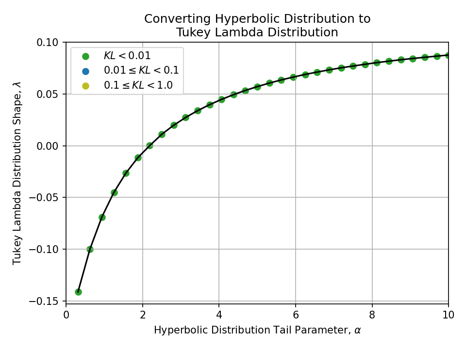
5. Hyperbolic distribution
   • Tails are controlled by tail parameter \(\alpha \in \mathbb{R}\)
   • \(\alpha \to \infty\) is a normal distribution
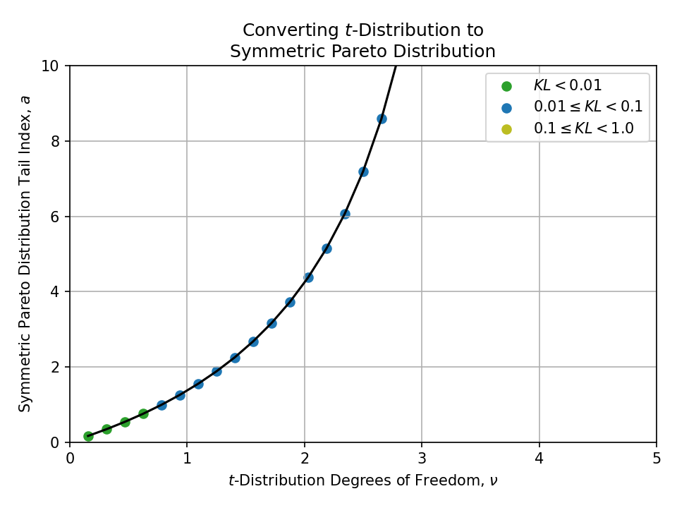
6. Symmetric Pareto distribution
   • Tails are controlled by tail index \(a > 0\)
   • This distribution is a strict power law and is never equal to a normal distribution. It becomes the Dirac delta function as \(a \to \infty\).
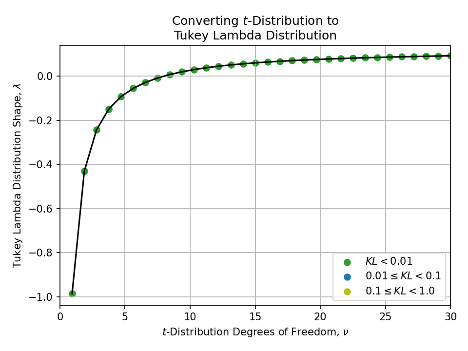
7. Tukey lambda distribution
   • Tails are controlled by shape \(\lambda \in \mathbb{R}\)
   • \(\lambda = -1\) is approximately Cauchy, \(\lambda \approx 0.14\) is approximately normal, and \(\lambda = 1\) is exactly uniform

Results

#

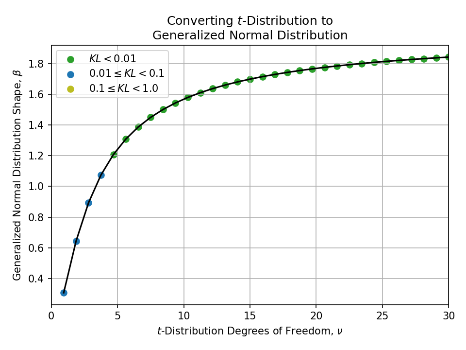
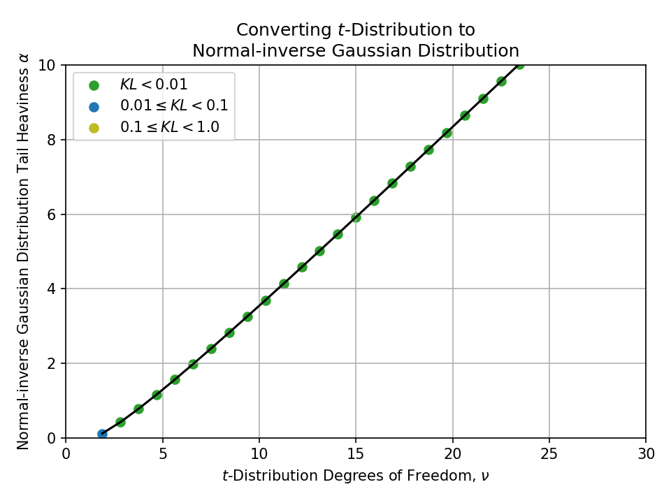
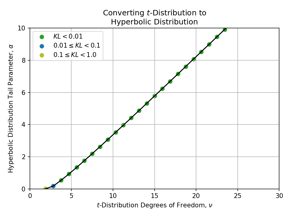
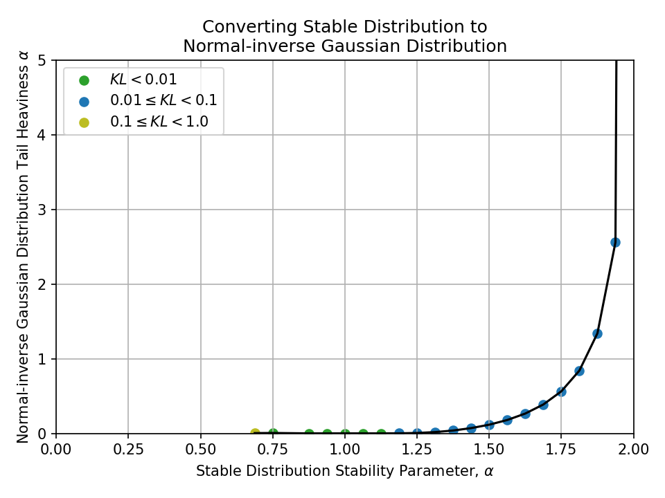
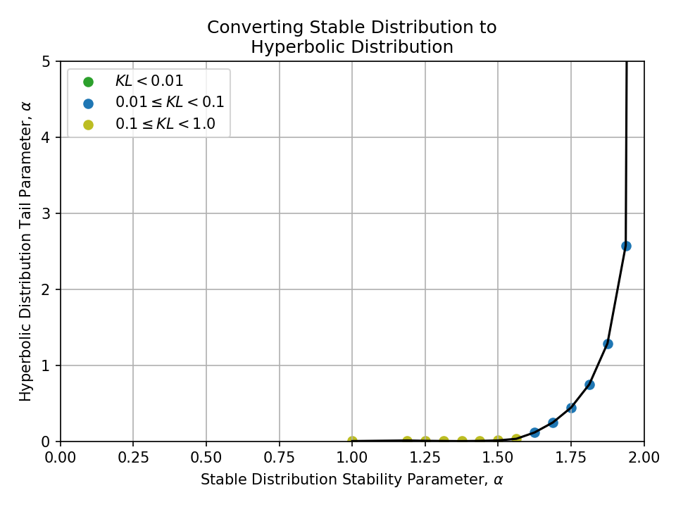
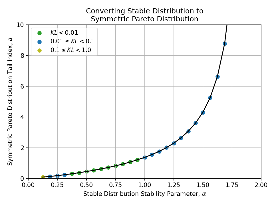
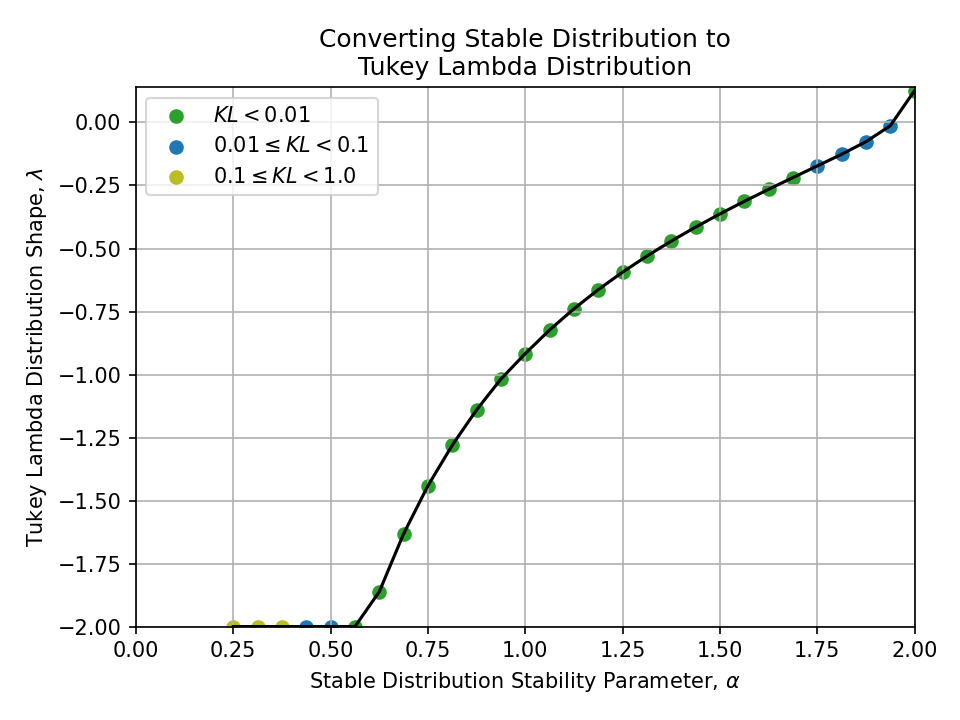
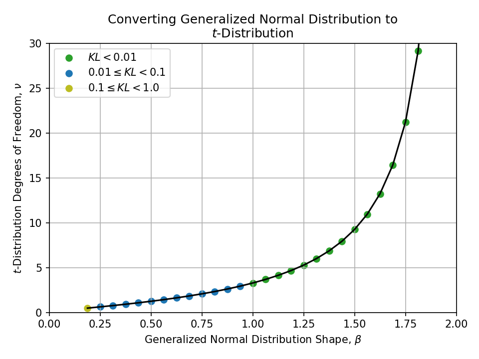
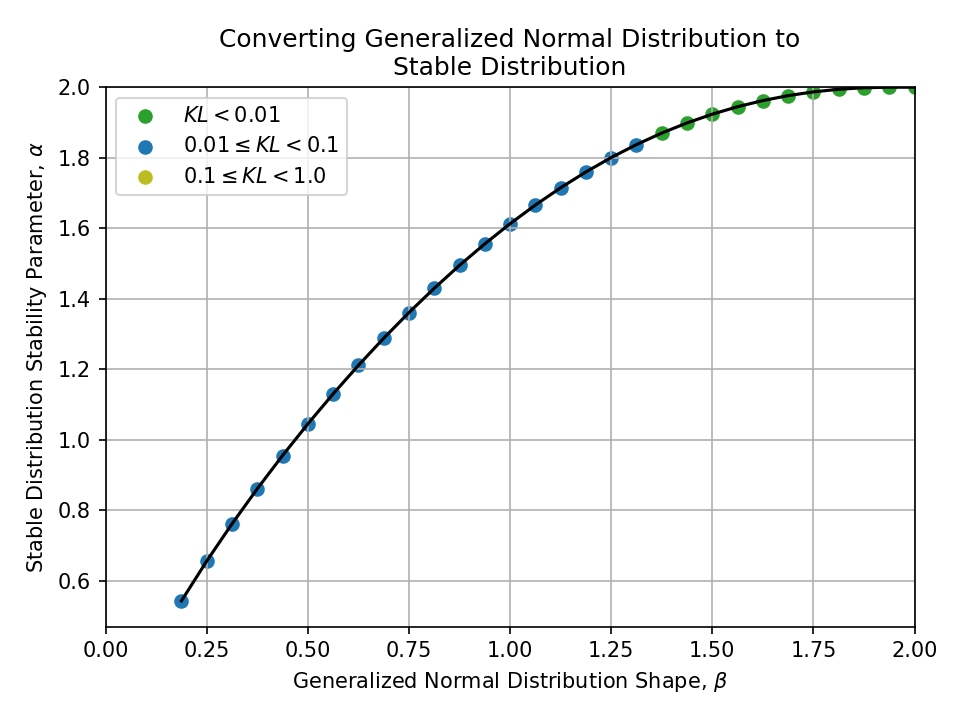
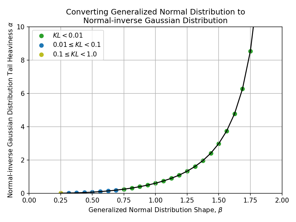
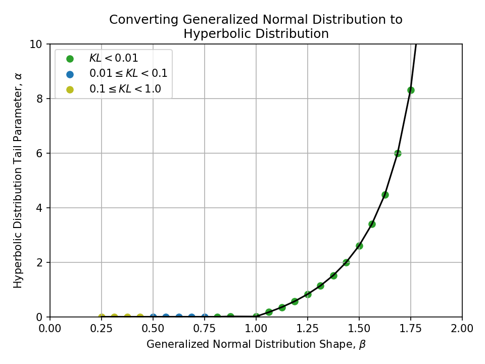
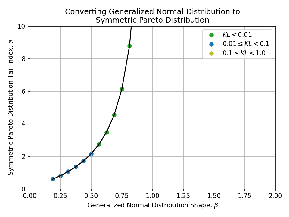
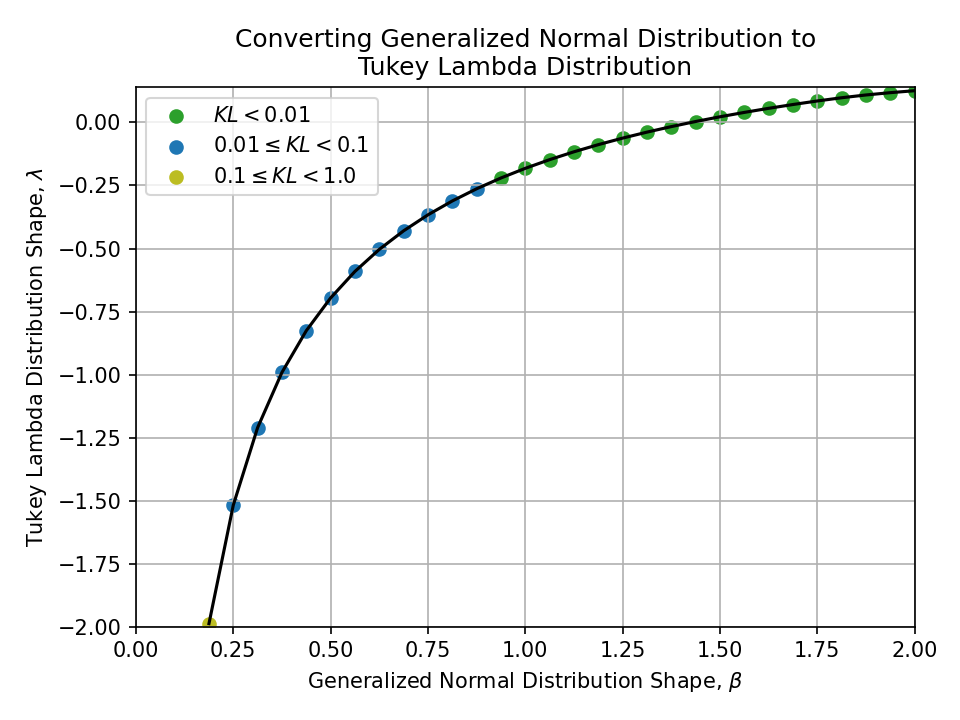
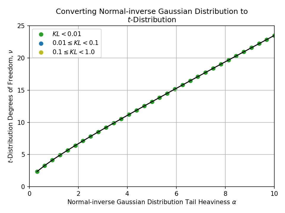
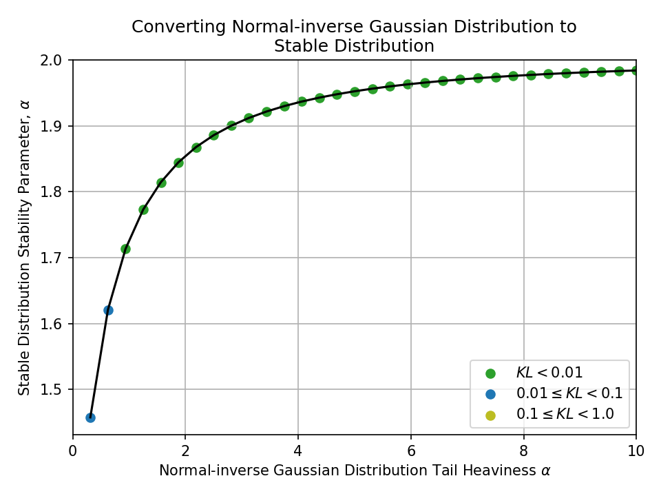
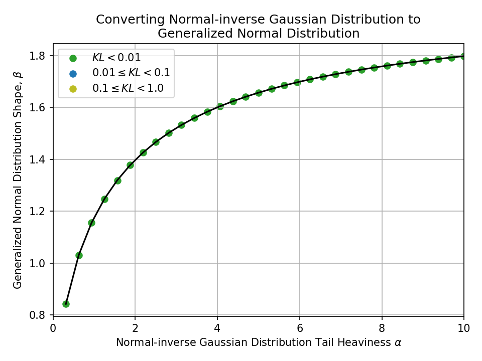
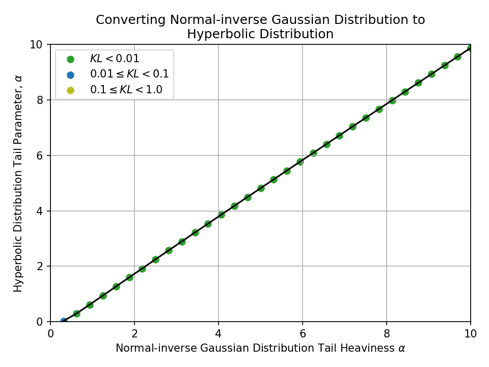
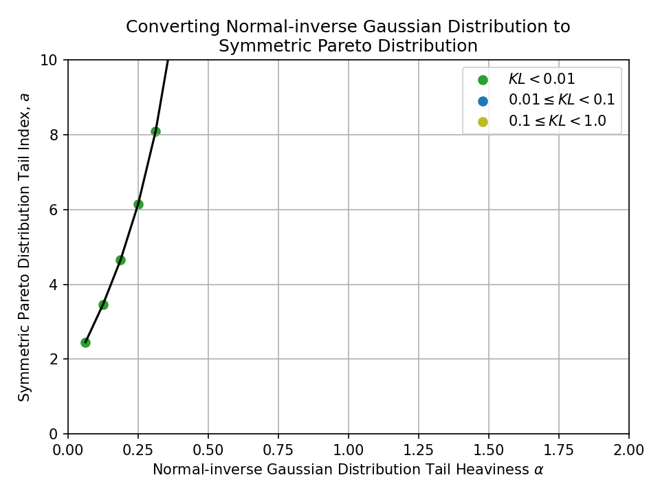
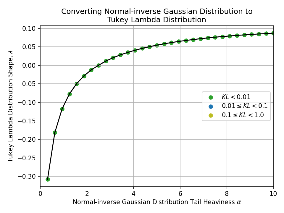
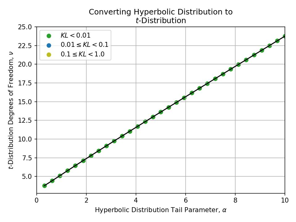
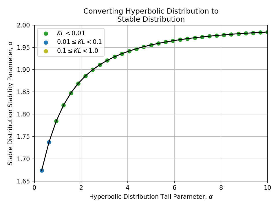
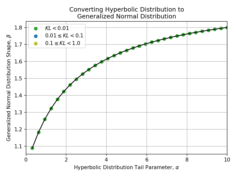
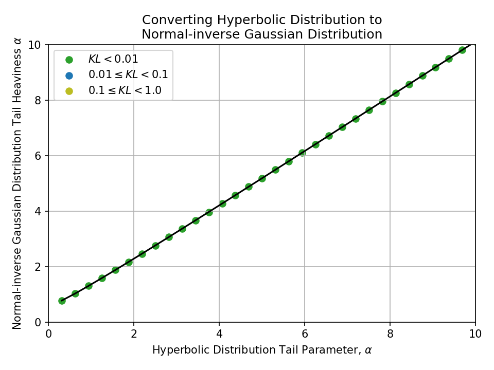
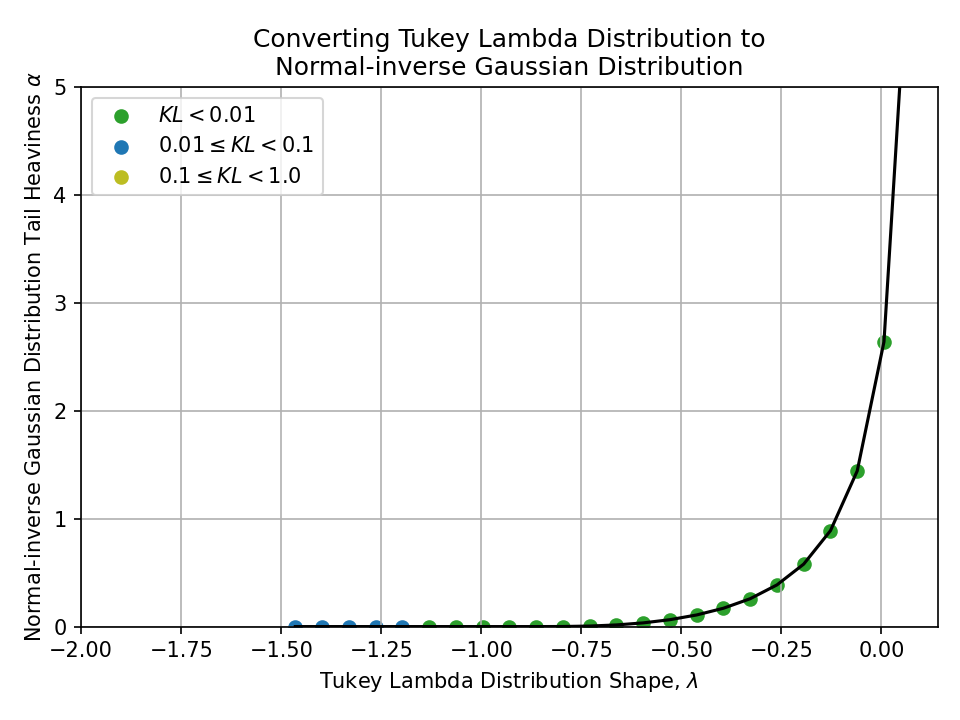
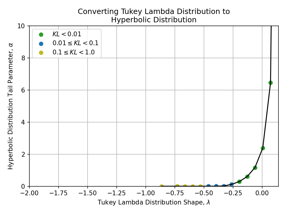
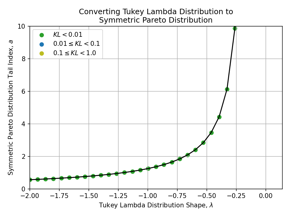
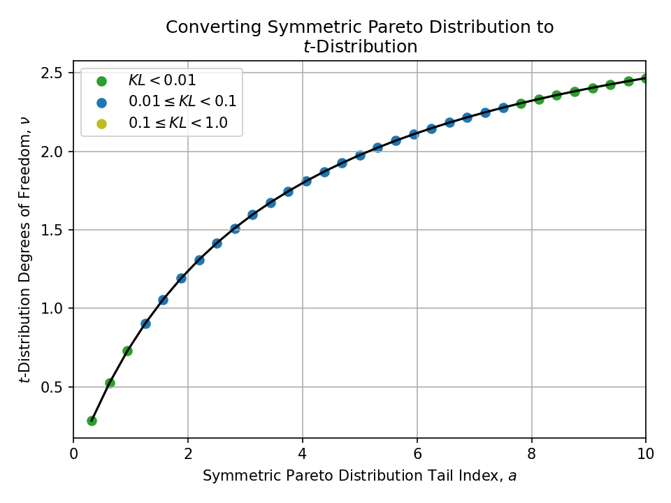
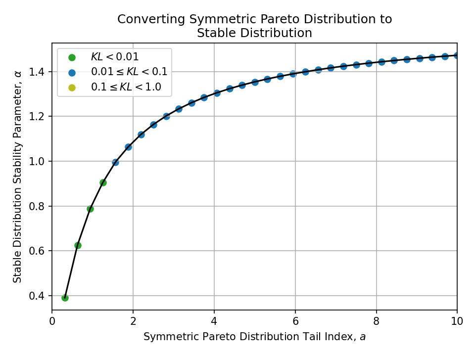
Below, I plot all conversions between pairs of the above distributions.

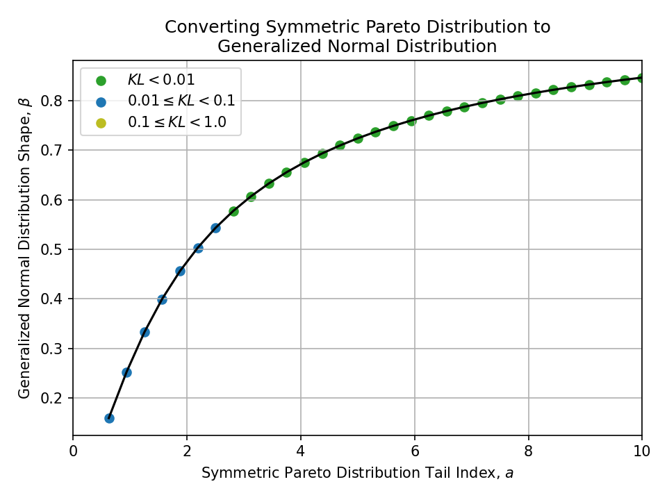
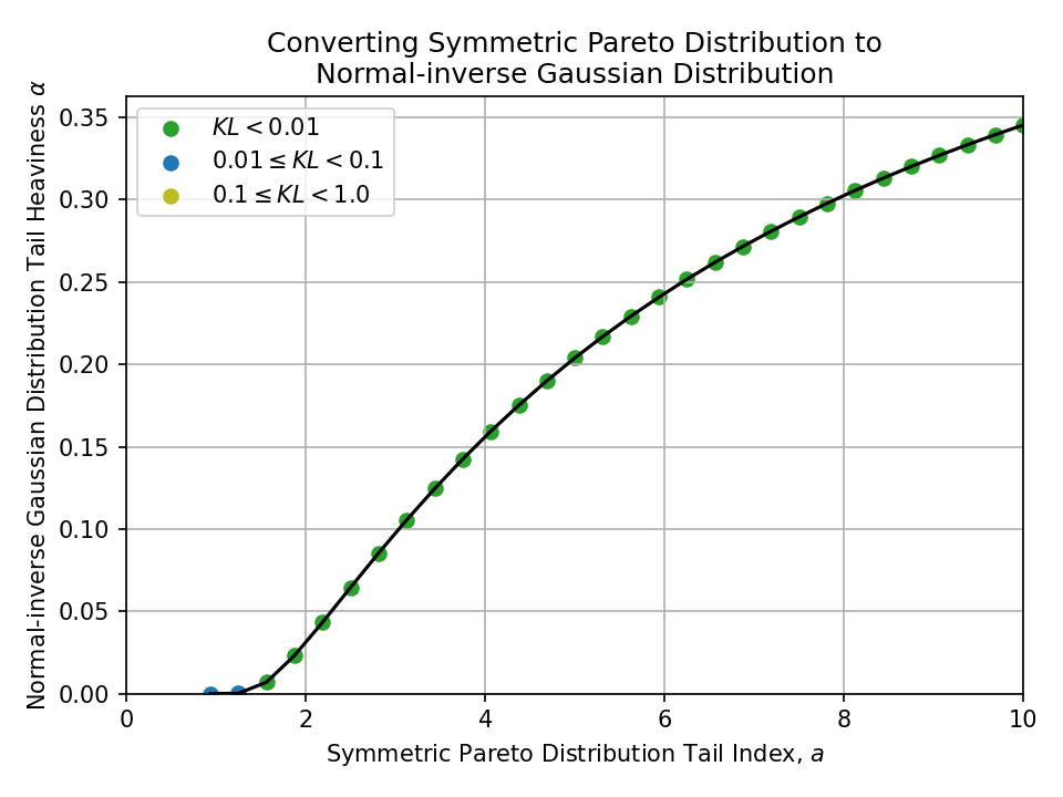
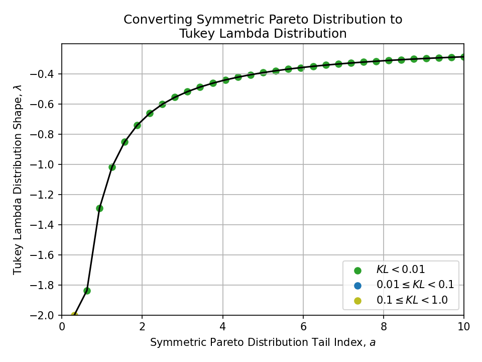
To better understand the quality of the conversions at a glance, the samples are colored

• Green \((KL < 0.01)\),
• Blue \((0.01 \leq KL < 0.1)\), and
• Yellow \((0.1 \leq KL < 1.0)\)

Nothing with a KL divergence above 1.0 is shown.

Converting from a t-Distribution

#

Click to expand

To a Stable Distribution

#

To a Generalized Normal Distribution

#

To a Normal-inverse Gaussian Distribution

#

To a Hyperbolic Distribution

#

To a Symmetric Pareto Distribution

#

To a Tukey Lambda Distribution

#

Converting from a Stable Distribution

#

Click to expand

To a t-Distribution

#

To a Generalized Normal Distribution

#

To a Normal-inverse Gaussian Distribution

#

To a Hyperbolic Distribution

#

To a Symmetric Pareto Distribution

#

To a Tukey Lambda Distribution

#

Converting from a Generalized Normal Distribution

#

Click to expand

To a t-Distribution

#

To a Stable Distribution

#

To a Normal-inverse Gaussian Distribution

#

To a Hyperbolic Distribution

#

To a Symmetric Pareto Distribution

#

To a Tukey Lambda Distribution

#

Converting from a Normal-inverse Gaussian Distribution

#

Click to expand

To a t-Distribution

#

To a Stable Distribution

#

To a Generalized Normal Distribution

#

To a Hyperbolic Distribution

#

To a Symmetric Pareto Distribution

#

To a Tukey Lambda Distribution

#

Converting from a Hyperbolic Distribution

#

Click to expand

To a t-Distribution

#

To a Stable Distribution

#

To a Generalized Normal Distribution

#

To a Normal-inverse Gaussian Distribution

#

To a Symmetric Pareto Distribution

#

No useful conversions found.

To a Tukey Lambda Distribution

#

Converting from a Symmetric Pareto Distribution

#

Click to expand

To a t-Distribution

#

To a Stable Distribution

#

To a Generalized Normal Distribution

#

To a Normal-inverse Gaussian Distribution

#

To a Hyperbolic Distribution

#

No useful conversions found, except the general observation that the Symmetric Pareto’s strict power law requires the Hyperbolic distribution’s tail parameter to be extremely small for a reasonable fit.

To a Tukey Lambda Distribution

#

Converting from a Tukey Lambda Distribution

#

Click to expand

To a t-Distribution

#

To a Stable Distribution

#

To a Generalized Normal Distribution

#

To a Normal-inverse Gaussian Distribution

#

To a Hyperbolic Distribution

#

To a Symmetric Pareto Distribution

#

See also and references

#

This analysis is mostly intended to be self-contained. Being able to look up these approximate tail parameter conversions is quite useful in practice!

These relationships become particularly relevant when:

• Comparing results across different papers, fields, or methods that tend to favor different distribution families
• Choosing which distribution to use based on computational or analytical tractability
• Demonstrating the robustness of a model to the choice of heavy-tailed distribution

For more details on the individual distributions, please see the Wikipedia pages linked throughout this post.