Modeling Stock Market Corrections Over 150 Years

Recently, Goldman Sachs claimed that the S&P 500 should deliver less than 1% annualized real returns over the next decade, partly due to the index having doubled in the last five years.

Their analysis was more nuanced (with error bars large enough to drive a truck through), but my initial reaction was pure skepticism. Is the stock market’s mean reversion really strong enough to do a Gambler’s Fallacy style prediction like this?

Indeed, such reversion is relatively weak. To see this, we’ll

1. Examine historical stock market data, and
2. Develop a stochastic model to analyze and forecast trends.

Looking at raw data

#

Data sets

#

For this analysis, I use two of the longest-running data sets available for major U.S. stock indices.

• Daily prices of the Dow Jones Industrial Average (“DJIA”) since February 1885,¹ and
• Monthly prices of the Real (inflation-adjusted) S&P Total Return Index (“S&P”) since January 1871.²

The DJIA data is especially valuable due to its granularity. However, it needs a few adjustments.

1. Data imputation: The New York Stock Exchange was closed for ~4.5 months in 1914 during the onset of World War I, leaving a lengthy gap in the data.

   Holiday and business day conventions have also changed over the centuries, creating inconsistent year lengths.

   To address both issues, I linearly interpolated to create a data set with values for every weekday in the time period.³

2. Adding dividends: The historical data does not represent a total return index, so I continuously added on the monthly dividend yields of the broader U.S. stock market.²

   I confirmed that this adjustment aligns closely with the official total return index that has been published since 1987.

These tweaks bring the DJIA in line with a nominal (not inflation-adjusted) total return index.

An aside on DJIA’s flaws

#

The Dow Jones Industrial Average is widely known to be a mediocre reflection of the total U.S. stock market.

It’s only composed of 30 large cap companies and is price-weighted, so high-priced stocks have an outsized impact on the index level, regardless of the size of the company.⁴

Despite this, DJIA’s long term returns closely track the broader stock market.⁵ This is my primary interest here, especially since I am most focused on long-term trends. Moreover, my total return adjustment uses the overall stock market’s dividend yield, which further mitigates the index’s shortcomings.

Historical 5Y returns

#

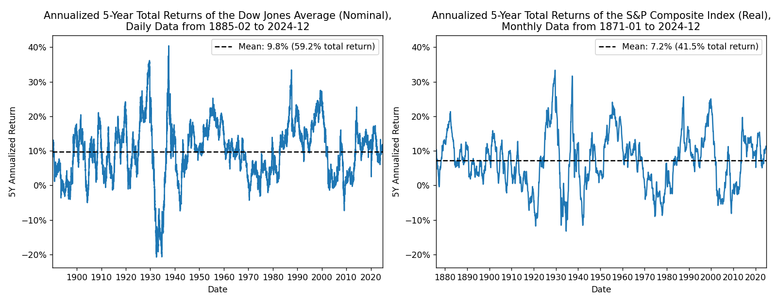
Plotting the historical returns of these indices reveal rough market cycles over time.

At a glance, it does seem plausible that periods of high returns are typically followed by periods of lower returns, and vice versa. This is precisely the concept of mean reversion.

However, we want to see a more explicit comparison of autocorrelation, the degree to which returns are correlated to previous values.

For this, it’s easier to directly visualize future returns against past returns.

Conditional 5Y returns

#

Here, we plot the next 5Y total return (y-axis) against the previous 5Y total return (x-axis).

Notably, mean reversion is only apparent following relatively huge market moves of say, \( {<}{-25\%} \) or \( {>}{125\%} \) returns in 5 years. Otherwise, the forward-looking average is not significantly different from a completely unconditional average.

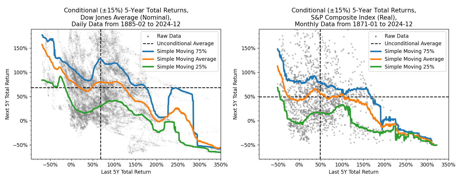
It’s worth noting that the far tails of the plot represent very sparse data. If you exclude the Great Depression (1930s), Black Monday (1987), and the Dot-com bubble (1990s), the observed range narrows significantly to around (-30%, +200%).

In any case, there is no clear evidence that a recent run of +100% should lead to a decade of zero growth.

In fact, research has shown that:

• Mean reversion in the stock market is so weak that it is often indistinguishable from random walk behavior.⁶
• It is mostly concentrated in periods of high economic stress and “virtually absent” when there is little economic uncertainty.⁷

Fitting a trend-reverting model

#

Estimating mean reversion is notoriously difficult due to its weak nature, but we can try to model it with a stochastic process. The sheer length of our data goes a long way in making calibration stable enough to be useful.

However, I warn that the analysis herein covers an extremely broad time period. As such, it is biased by economic crisis outliers and ignores the possibility that mean reversion has weakened over time, particularly as markets have become more efficient.

Additionally, keep in mind that all returns discussed are nominal and not adjusted for inflation.

Choosing a model

#

The most straightforward mean-reverting model is the Ornstein-Uhlenbeck process, $$ dr_t = -\theta\left(\mu - r_t\right) dt + \sigma dW_t $$ This has returns \( r_t \) reverting back to a long-term average, \( \mu \), with reversion speed controlled by \( \theta \).⁸

However, I would like to enhance it in a few ways.

1. Fat tails and skew: I replace the Brownian motion term, \( dW_t \), with a stable Lévy process, \( dL_t^{\alpha, \beta} \). This better fits the empirical fat-tailed and right-skewed nature of stock market returns, which simple normal distributions cannot capture.

   This also prevents the calibration “overestimating \(\theta\)” in order to fit the data more closely.

   Importantly, this distribution is analytically intractable, which is a significant but not insurmountable complication.⁹

2. “Trend reversion”: The whole point of this analysis is to perform an estimate that assumes stocks will revert back to a global (exponential) price trend rather than just have returns reverting back to a long-term average.

   Luckily, this makes the effect of the reversion parameter more pronounced and thus easier to estimate.

   To be clear, I do not think this is a particularly good assumption, but it is precisely the thought that kicked off this whole experiment.

As such, we use the following stochastic process, which I’ll refer to as Stable Trend-Reverting Ornstein-Uhlenbeck (“STROU”). $$ dr_t = \mu \cdot dt + \theta\left(\mu \cdot t + \hat{r_0} - r_t\right) dt + \sigma dL_t^{\alpha, \beta} $$ where the actual price level follows \( S_t = S_0 \exp(r_t) \).

This process is parameterized by

• \(\alpha \in (0, 2]\), which controls the fatness of the noise term’s tails (\(\alpha=2\) is a normal distribution, with smaller values giving fatter tails)
• \(\beta \in [-1, 1]\), which controls the skew of the noise term (\(\beta = 0\) has no skew)
• \(\sigma\), the scale of the noise term. This tends to decrease as \(\alpha\) decreases since that also “widens” the distribution
• \(\mu\), the long-term drift of the process and global trend towards which the returns revert
• \(\hat{r_0}\), an estimate for calibration convenience of the process’s starting point relative to the global trend

In other words, \(\alpha, \beta, \sigma\) control the distribution of the noise term and the returns revert back to a long-term \( \mu \cdot t + \hat{r_0} \) trend based on speed \( \theta \).

Calibrating the model

#

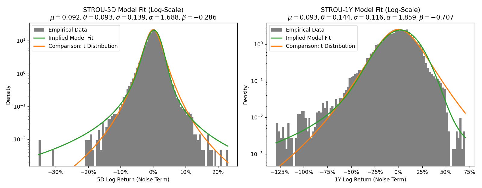
I calibrated two versions of models in a simple MLE-like manner,¹⁰ each capturing different features of the data.

• STROU-5D, calibrated to 5-day returns, yielding \( \mu \approx 0.092, \theta \approx 0.093, \sigma \approx 0.139, \alpha \approx 1.688, \beta \approx -0.286 \).
  • This version should better capture short-term volatility at the expense of long-term trend reversion
  • Hence, this has lower \( \alpha \) (fatter tails) but lower \( \theta \) (weaker reversion)
• STROU-1Y, calibrated to 1-year returns, yielding \( \mu \approx 0.093, \theta \approx 0.144, \sigma \approx 0.116, \alpha \approx 1.859, \beta \approx -0.707 \).
  • This should better capture long-term trend reversion at the expense of short-term volatility
  • Hence, this has higher \( \alpha \) (thinner tails) but higher \( \theta \) (stronger reversion)

In both cases, the global trend is similar and corresponds to an expected nominal annualized return of \( \left[\exp(0.0925)-1\right] \approx 9.7\%\).

Plotting the returns against the model distributions shows quite a good fit overall.

Plotting example simulations

#

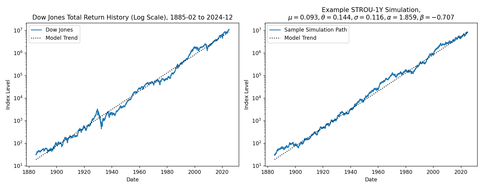
We can plot an example simulation to show that these models are reasonable. The sampled random variates are identical in both cases so that they can be compared directly.¹¹

Here, the higher volatility of the 5-day calibration is readily apparent, and both models look reasonable enough.

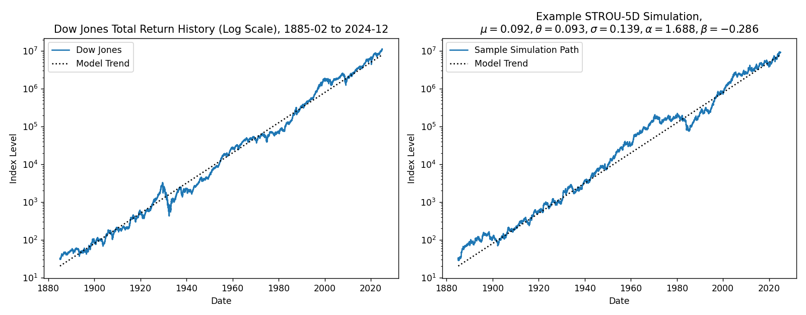
Especially around 1980 in the simulations, you can see the effect of the fatter tails from the STROU-5D simulation compared to STROU-1Y.

Analyzing modelled conditional returns

#

Given the calibration above, we can analyze the models’ distribution of returns for the next 5 years given the prior 5 years. To align with the global long-term trend, we show the average implied by the model’s log returns here.

Obviously, the plot is similar to an exponential fit of the conditional 5Y returns that we plotted earlier and indeed matches quite well in the typical ranges experienced by the stock market.

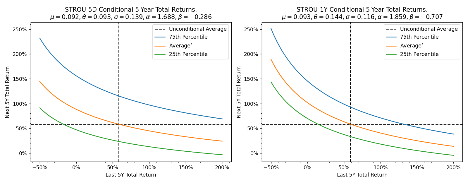
Again, we can see that a +100% return does not bring about a subsequent period of zero growth.

These models actually imply that a +100% 5-year return would on average be followed by

• STROU-5D: around +45% in 5 years (+8% annualized)
• STROU-1Y: around +40% in 5 years (+7% annualized)

This translates to a 10-year return of approximately +180-190% (+11% annualized).

Indeed, plotting out the same curves with annualized returns shows this more clearly. The trend reversion is simply not strong enough to zero out the next 5 years of expected growth.

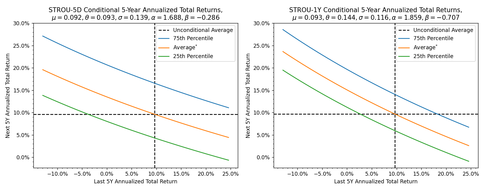
On the other hand, the far tails are probably not very realistic. For instance, the models imply a prior 5-year return of -50% would on average be followed by

• STROU-5D: around +140% (+19% annualized) for a 10-year return of +20% (+2% annualized)
• STROU-1Y: around +190% (+24% annualized) for a 10-year return of +45% (+4% annualized)

Regardless, we can be pretty confident that mean reversion alone is not sufficient to make Goldman’s prediction.

See also and references

#

Most of the content in this post is intended to be self-contained, but I would encourage looking through the numerous resources linked in the body and footnotes of this post.

In particular,

• The datasets: Dow Jones history from MeasuringWorth and Robert Shiller’s U.S. Stock market data
• Mean reversion research papers: Poterba et al. and Spierdijk et al.
• General stochastic modelling introductions on Wikipedia: Stochastic Process, Lévy process, Ornstein-Uhlenbeck process, Itô calculus, etc.