
When building out a new computer, it is relatively easy to calculate which choices would be most efficient in terms of performance per dollar.
But how quickly will that performance degrade relative to newer systems entering the market? What if you expect to recover some of those funds by selling components once you upgrade? Is there an optimal frequency for upgrading components? Is it possible to “future-proof” a system?
These questions require a deeper analysis into historical data to understand how computer performance changes over time and relates to build cost.
The data set #
To study the overall state of PC builds through time, we
- Scraped the last ~11 years of build recommendations from Logical Increments and adjusted the prices for inflation.1 In general, they provide component suggestions across a wide range of " tiers" (budgets).
- Pulled a complete set of CPU and GPU benchmarks from PassMark, assigning half weight to both components when evaluating overall system performance.2
Below, we plot the historical trend of build prices and performance across many of the tiers.
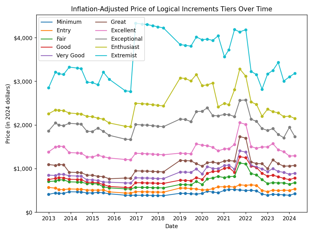
Overall, the prices are quite stable across time for most tiers, with the notable exception of the spike during the global chip shortage and cryptocurrency mining boom of 2021.
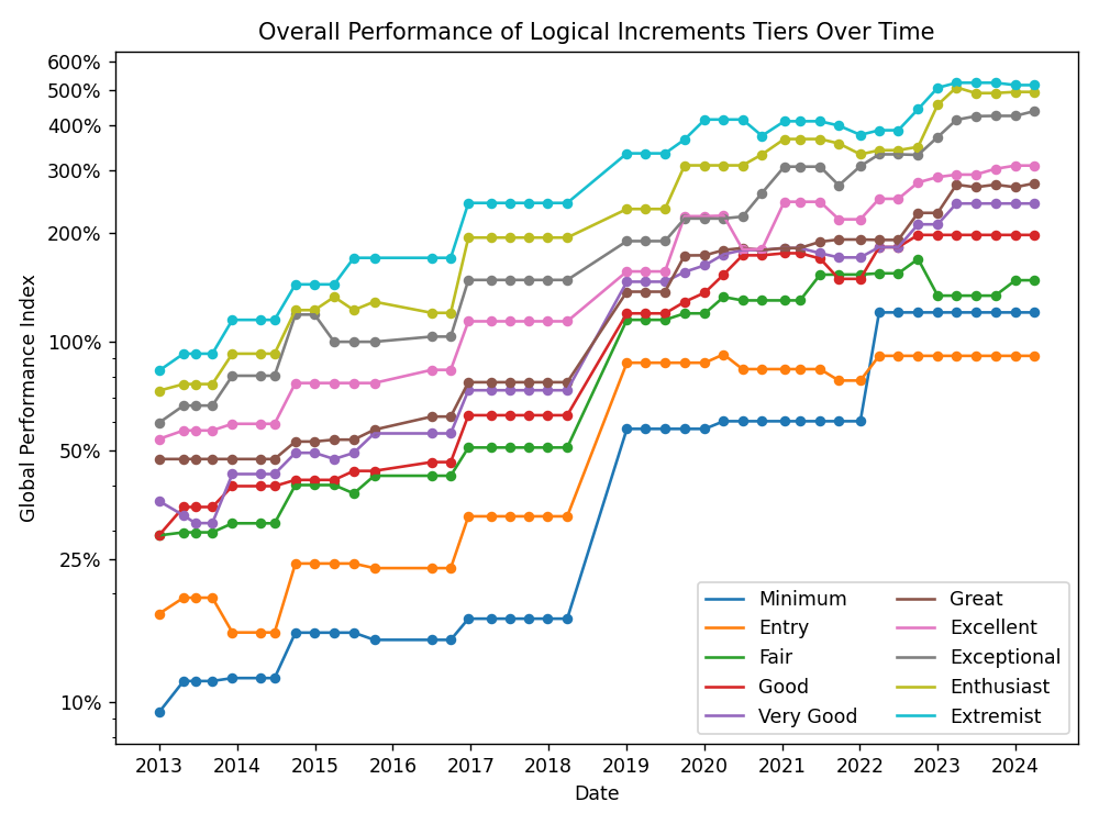
Similarly, build performance shows a steady increase over time, which is depicted below.3
More details and the data itself can be found in “Historical PC Build Data”. Next, we’ll derive some model assumptions from this data.
Model assumptions #
Fundamentally, our model aims to project PC performance over time, which will tell us the relative speed of obsolescence between older and newer builds. Separately, we’ll fit estimates of build performance against total component cost.
This will rely on two basic assumptions.
1) Computer performance improves at a constant rate, regardless of cost #
Our model operates under the assumption that computer performance experiences a consistent rate of improvement over time, regardless of the initial cost of the components. This is supported by the fact that our plots of log-performance show a roughly linear trend across time for all tiers.
Moreover, it is a reasonable assumption that computer chip fabrication techniques fundamentally improve simultaneously across all consumer cost ranges. Indeed, low-end and mid-end components are often just binned versions of their high-end counterparts.
Our fit to the data is shown below, and appears quite reasonable.
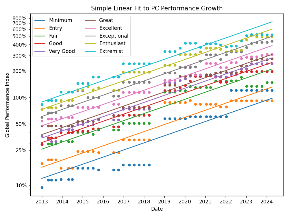
We’ll only use the slope (performance growth rate) here. However, it’s important to acknowledge a few limitations and nuances.
- There is considerable noise at lower end of the performance spectrum, partially due to recent GPU supply issues and sporadic significant improvements in cheaper components.
- There is some tapered growth at the higher end, partly due to the phase-out of SLI setups, which somewhat inflates the performance of older high-end builds.4
Despite this, the overall fit provides a useful rule of thumb, particularly within the Fair to Exceptional tiers. Those tiers span builds that cost around $700 to $2000, which contains practically the entire range of decent performance per dollar.
2) We can predict computer performance from component cost alone #
Our model also assumes that computer performance can be predicted solely from the cost of its components, which is a direct consequence of all tiers improving at the same rate.
This is also based on the desire to translate between a build’s price and its corresponding performance.
Importantly, these performance values are normalized against those from the same time period, allowing for meaningful comparisons across time. In other words,
- 100% on the “Global Performance Index” from the earlier plots is roughly the performance of a mid-end system from 2019.5
- 100% on the “Time-Specific Performance Index” in the plots below indicates performance comparable to the average build from the same time period.6
Below, we plot the relationship between performance and price. I encourage you to consider what functional form would work best here. Clearly, it must be monotonic, but what other features of the data should be captured?
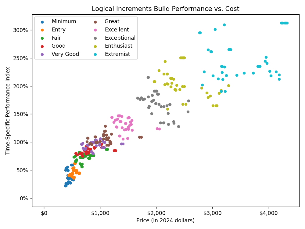
To me, it is clear that there is very rapid improvement per dollar for cheaper tiers, and this slows to a heavily heteroskedastic and roughly-linear trend.
Naturally, I also wanted the function to pass through the origin (as spending zero money yields zero performance), so I settled on a tweaked logistic function with a linear asymptote.
$$ f(x) = \frac{a}{1 + b \cdot \exp(-c \cdot x)} + d \cdot x - \frac{a}{1+b} $$
The plot below displays the result of a least squares fit with this function, providing performance as a function of price. Importantly, the fit was actually applied to log-performance data to address the heteroskedasticity.
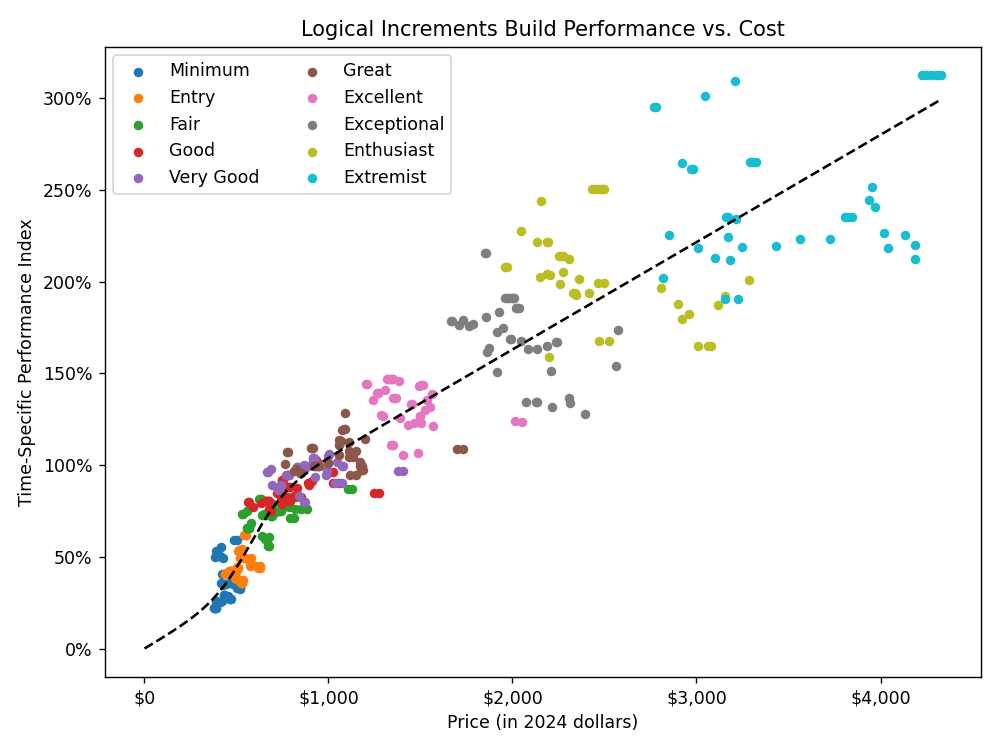
As with the earlier fit, this appears to be quite good overall. However, there’s some inconsistency across time in the data for costs exceeding ~$2000, so I would caution interpreting predictions beyond that point.
Model results #
Now, we can explore the modeled answers to the questions that we started with.
To do so, we take a simple approach to planning future upgrades.
- The CPU and GPU are upgraded with a fixed frequency, which necessitates upgrading the motherboard and RAM as well to support potential socket changes.
- If used components are resold, we assume they yield 2/3rds of the price of an equivalent new component, accounting for overall computing improvements since the original purchase date.
- All other components, such as storage and power supplies, are assumed to have a longer lifespan and are replaced once per decade.
What is the optimal amount to spend on a new build? #
Answering this question fundamentally depends on whether you except to recoup any money from future upgrades through the sale of your used components. If not, it is quite common to gift older builds to relatives or repurpose them as secondary systems.
If not planning to resell used components #
In this scenario, the decision boils down to a straightforward calculation of performance per dollar.
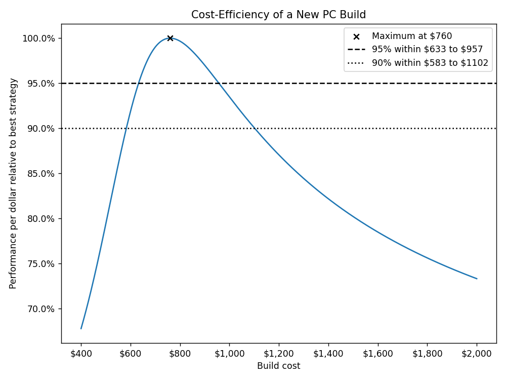
Unsurprisingly, the optimal price point is right around what we’d typically refer to as “mid-range”.
However, it’s noteworthy that a wide range of prices yield quite close to optimal performance per dollar. In fact, pretty much anything other than high-end and enthusiast builds are within 10% of the best cost efficiency possible.
If planning to resell used components #
To motivate the range of PC upgrading strategies here, let’s consider three approaches.
- Upgrading a $500 PC every 2.5 years
- Upgrading a $1000 PC every 5 years
- Upgrading a $2000 PC every 10 years
Below, we plot the effective performance of all three builds relative to then-current systems.
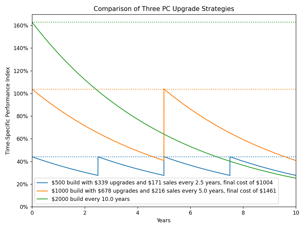
Comparing these strategies should reveal a few interesting insights.
- The $1000 build offers more than twice the performance of the $500 build for less than 50% extra cost.
- The $2000 build’s performance falls below the $1000 build after year 5 and both builds after year 7.5. This is likely to be an unacceptable outcome, especially for users expecting their initial, enthusiast-level performance.
That said, it’s not immediately clear which of the first two strategies are most cost-effective or what that should even mean in this temporal context!
As such, we’ll consider cost-effectiveness as the average performance of each system per dollar and plot the results of all possible choices below.7
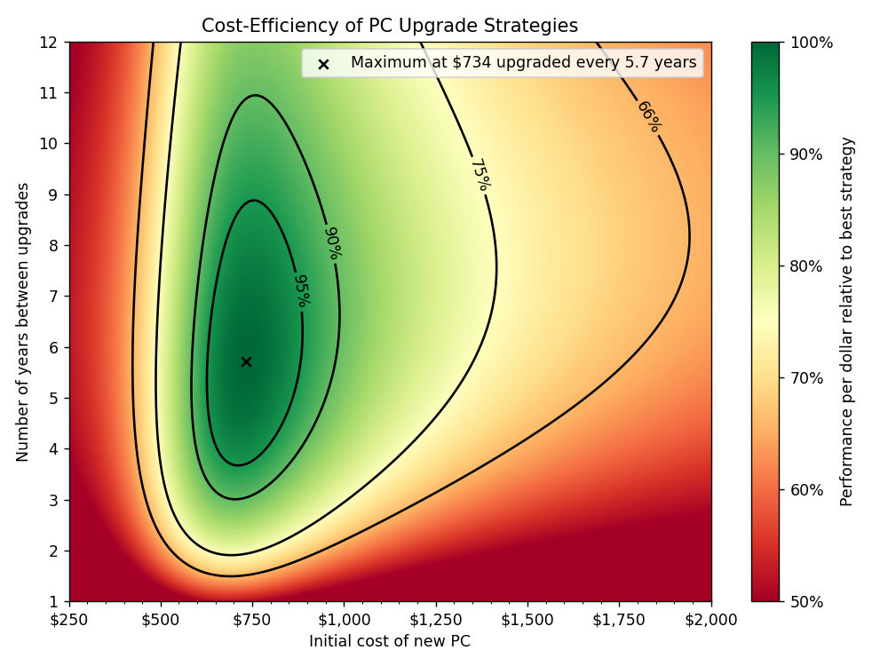
Interestingly, the optimal price point has actually fallen slightly compared to considering a new PC build in isolation! There is an interesting trade-off here.
- The longer you wait between upgrades, the more time your build’s performance will degrade, but
- The longer you wait between upgrades, the more performance you can buy for the same fixed dollar amount
Again, note how much leeway you have while still having extremely high cost-efficiency! There is a huge range with prices between ~$600 and ~$1000, and an upgrade frequency above 3 years that are within 10% of the best cost efficiency possible.
How much do you need to spend to “future-proof” a new build? #
In general, “future proofing” a PC is ill-advised. It is significantly more cost-effective to purchase a moderately powerful system and plan on periodic upgrades, as we saw above.
Nevertheless, many new PC builders are tempted by this idea, so let’s explore what it would actually take. In contrast to our earlier analysis focusing on average performance, here we are interested in the minimum performance of a system over time.
In other words, we’re interested in targets such as “I always want at least a Great build, compared to current systems, for the least cost possible.” Optimizing this metric yields the following build strategies.
| Performance Target | Optimal Strategy |
|---|---|
| Minimum (~35%) | $650 build upgraded every 3.7 years |
| Entry (~45%) | $709 build upgraded every 3.0 years |
| Fair (~72%) | $927 build upgraded every 1.7 years |
| Good (~85%) | $1259 build upgraded every 1.8 years |
| Very Good (~96%) | $1648 build upgraded every 2.1 years |
| Great (~105%) | $1942 build upgraded every 2.2 years |
| Excellent (~132%) | $2764 build8 upgraded every 2.4 years |
| Exceptional (~170%) | $3861 build upgraded every 2.5 years |
You can immediately see from the relatively short upgrade frequencies that this “future proofing” is a less cost-effective focus. Remember, we optimized for lowest cost, so longer time periods would be even more costly.
Additionally, note how the number of years between upgrades drops sharply as we move beyond the point of highest cost efficiency.
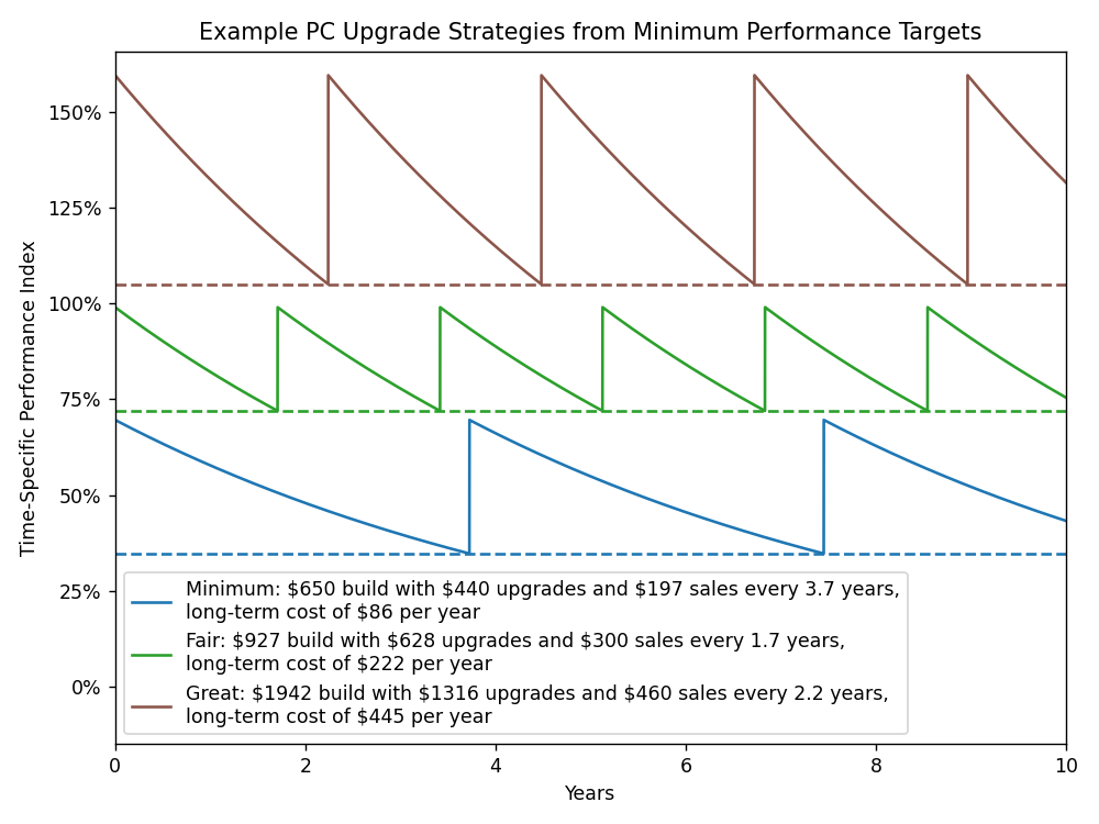
Another way to interpret this data is to compare each strategy to its equivalent with the same average performance. The latter are all more cost-effective, albeit with an average of ~30% larger performance swings, starting out faster and ending up slower between each upgrade.
| Tier Name | Optimal Minimum Performance Strategy | Equivalent Average Performance Strategy |
|---|---|---|
| Minimum | $650 build upgraded every 3.7 years, $440 upgrades and $197 sales, long-term cost of $86 per year | $734 build upgraded every 5.7 years, $498 upgrades and $173 sales, long-term cost of $81 per year |
| Entry | $709 build upgraded every 3.0 years, $481 upgrades and $228 sales, long-term cost of $108 per year | $804 build upgraded every 4.5 years, $545 upgrades and $209 sales, long-term cost of $100 per year |
| Fair | $927 build upgraded every 1.7 years, $628 upgrades and $300 sales, long-term cost of $222 per year | $1273 build upgraded every 4.0 years, $862 upgrades and $260 sales, long-term cost of $191 per year |
| Good | $1259 build upgraded every 1.8 years, $853 upgrades and $346 sales, long-term cost of $320 per year | $1950 build upgraded every 5.3 years, $1321 upgrades and $266 sales, long-term cost of $261 per year |
| Very Good | $1648 build upgraded every 2.1 years, $1117 upgrades and $400 sales, long-term cost of $392 per year | $2576 build upgraded every 6.1 years, $1745 upgrades and $276 sales, long-term cost of $325 per year |
| Great | $1942 build upgraded every 2.2 years, $1316 upgrades and $460 sales, long-term cost of $445 per year | $3051 build upgraded every 6.5 years, $2067 upgrades and $287 sales, long-term cost of $374 per year |
As with all models, you should take this analysis as a rough guideline and factor in your own special considerations in your plans. Do some of your own research!
You’re bound to find a special deal or unusually cheap offer, which will necessarily deviate from the predictions shown here. Any big upcoming hardware announcements could also warrant briefly delaying an upgrade.
See also and references #
- For additional details and access to the dataset used in this analysis, refer to “Historical PC Build Data”.
- PCPartPicker, an invaluable resource for planning out PC builds, offering customizable component selections, simple compatibility checks, price discovery, and many useful product filters. They also provide their own series of recommended build guides as well as a massive repository of community builds.
- The resources, advice, and support available at /r/buildapc, which is an online community dedicated to custom PC assembly.
- The inline linked Wikipedia articles on the 2020-2023 global chip shortage, product binning, SLI, logistic functions, and heteroskedasticity.
- Our data scraping sources, Logical Increments and PassMark, with help from the Internet Archive.
I accept that Logical Increments is not really a gold standard in terms of optimal PC builds, but it is quite good as a rough guideline, especially since we are moreso concerned with relative improvements in performance over time. ↩︎
Similarly, PassMark’s methodologies are definitely not perfect and have some biases, but they should be fine for comparing relative changes over time. ↩︎
The increase is “steady” in an exponential sense, note the logarithmic scale in the plot. ↩︎
Whether SLI actually improves performance depends heavily on the use case and is beyond the scope of this discussion. Generally, it can either scale up perfectly, degrade performance compared to a single GPU, or fall somewhere in between. ↩︎
Indeed, the automatically computed baseline here is somewhere around pairing an i7 7700K with an RX 470, which is not far off from the Ryzen 5 2600 + RX 570 builds of 2019. ↩︎
Really, “average” here means the geometric mean since the tiers’ prices roughly increase in constant ratios, not constant dollar amounts. ↩︎
This is much more subtle than you might expect. Computer performance improvement, and degradation relative to future systems, is exponential. Then, the normalization of cost must include the initial system price, the costs of future upgrades, and the funds recouped from selling older components. Moreover, these should all be adjusted for inflation, but that is already baked into our analysis at this point. ↩︎
Again, don’t put too much emphasis on any of the builds that are this expensive. Builds beyond ~$2000 do not have very stable properties across time. ↩︎