A Simple Derivation of the Black-Scholes Option Pricing Formula

The discovery of the Black-Scholes-Merton formula for pricing options in 1973 was one of the most important breakthroughs in modern financial history, earning two of its authors the Nobel Memorial Prize in Economic Sciences and leading to a huge increase in options trading volume.

The traditional derivation involves

1. Constructing a particular hedging portfolio that eliminates all risk from the option,
2. Realizing this implies a stochastic differential equation,
3. Imposing boundary conditions based on the option’s payoff, and
4. Analytically solving via a change of variables.

Needless to say, this requires at least undergraduate-level knowledge of stochastic calculus, differential equations, and financial hedging.

However, there is an alternate derivation that is accessible to anyone familiar with basic probability and statistics.

I’ve found this is much more straightforward to explain to those without a finance background, so I’ve outlined the argument below.

Here, I’ll be moving integral calculations to the footnotes as people are usually happy enough deferring to a symbolic integrator or simply knowing that they could be solved without much trouble.

What even is an option?

#

The most basic option gives you the right to buy a stock at a specific price (the “strike price”) on a certain date in the future.¹

So, buying a “call option for Apple Inc. with strike $300 expiring on 7/15/2025” means that on the expiration date:

• If Apple’s stock price goes to \(S > \$300\), you make \(\left(S - \$300\right)\)!

  In effect, you exercise your right to buy the stock from the seller at $300 and then immediately sell it in the market for \(S\).

• If Apple’s stock price goes to \(S < \$300\), you make nothing, but you also don’t lose anything!

After taking the price of the option itself (the “premium”) into account, this is what your profit looks like for various final prices of Apple’s stock.

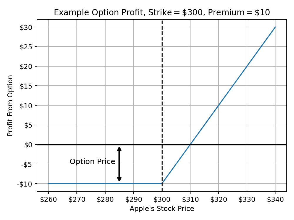
How would you assign a fair price for this?

#

One thing I want to make clear is it’s not obvious how much you should charge for an option. The buyer makes a profit based on the (unknown) stock price in the future!

In fact, before Black-Scholes, option pricing was somewhat based on vibes.² So much so that Ed Thorp made tens of millions of dollars exploiting mispriced options after discovering his own pricing formula years before Black-Scholes was published.

However, if we could just simulate the stock price at that time, then

1. We could compute the average amount of profit the buyer would make from the option as in the profit diagram above (ignoring the premium), and
2. Charge that same amount for the option price

Then on average, neither the buyer nor the seller makes any profit. That’s fair!

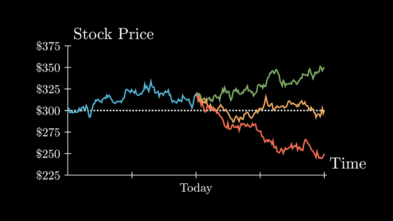
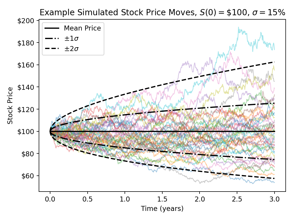
So, how would you simulate a stock price?

#

Luckily, this is where Black-Scholes makes a huge simplifying assumption. Define \(S(t)\) as the (distribution of the) stock price after \(t\) years.

Then, assume that the stock’s log returns \(\ln\left(\frac{S(t)}{S(0)}\right)\) follow a normal distribution!

Why logarithms?

#

The question I often get here is “why do these returns involve a logarithm? Isn’t it more intuitive to just say that, e.g., an increase from $100 to $150 is a return of \(\left(\$150 / \$100\right) - 1 = {+}50\%\)?”

The most reasonable way to counter this is that a normal distribution would assign nonzero probability to returns less than -100% and thus negative stock prices, which is not realistic.

Moreover, the logarithm encodes the fact that returns are multiplicative, not additive! Remember,

• If a $100 stock goes up 10% twice, it goes to \((1.1 \cdot 1.1 \cdot \$100) = 1.1 \cdot \$110 = \$121\) for a total return of 21%.
• If a $100 stock goes down 10% twice, it goes to \((0.9 \cdot 0.9 \cdot \$100) = 0.9 \cdot \$90 = \$81\) for a total return of -19%.

Using the logarithm naturally resolves this asymmetry quirk by converting the multiplications to additions since \(\ln(x \cdot y) = \ln(x) + \ln(y)\).

Considering the distribution of \(S(1)\)

#

Now, let’s return to the distribution of stock returns and prices. Looking at \(t=1\) for simplicity, $$ \begin{aligned} \ln\left(\frac{S(1)}{S(0)}\right) &\sim N\left(\mu, \sigma^2\right)\\ S(1) &\sim S(0) \cdot \exp\left(N(\mu, \sigma^2)\right) \end{aligned} $$

We’ll take \(\sigma\) to be the standard deviation of annual stock returns, but what should \(\mu\) be?

Determining the normal distribution’s \(\mu\)

#

Really, we don’t want our simulation to be biased towards the stock increasing or decreasing on average, so we need to figure out what choice of \(\mu\) keeps \(\mathbb{E}[S(1)] = S(0)\).

If we just keep \(\mu = 0\), we can find the bias by determining the PDF of that exponential term³ and computing a simple integral.⁴ $$ \begin{aligned} \mathbb{E}[S(1)] &= \mathbb{E}\left[S(0) \cdot \exp\left(N\left(0,\sigma^2\right)\right)\right]\\ &= S(0) \cdot \int_0^{\infty} x \cdot f_{\exp\left(N\left(0, \sigma^2\right)\right)}(x) \text{ d}x\\ &= S(0) \cdot \exp\left(\frac{\sigma^2}{2}\right) \end{aligned} $$ Okay, that drifts the normal distribution upwards by \(\sigma^2 / 2\)!

We’ll need \(\mu = -\sigma^2 / 2\) to counteract that.

Fully determining the distribution of \(S(t)\)

#

Now, we have $$ S(1) = S(0) \cdot \exp\left(N\left(-\frac{\sigma^2}{2}, \sigma^2\right)\right) $$ So, the distribution of stock returns after \(t\) years is just $$ \ln\left(\frac{S(t)}{S(0)}\right) \sim N\left(-\frac{\sigma^2}{2}\cdot t, \sigma^2 \cdot t\right) $$ The reasoning here is exactly the same as why \(\left[N\left(0,\sigma^2=1\right) + N\left(0,\sigma^2=1\right)\right] \sim N\left(0,\sigma^2=2\right)\).

Note that upward price moves tend to be larger than downward ones! A simple way to see why this is the case is that doubling $100 twice increases it to $400 while halving $100 twice only decreases it to $25.

Now that we have the \(S(t)\) distribution, we could just run a simulation and calculate the average amount of profit for the option.

And we don’t need to do a simulation at all!

#

One of the points of taking the returns to be normally distributed is so that everything can be computed analytically.

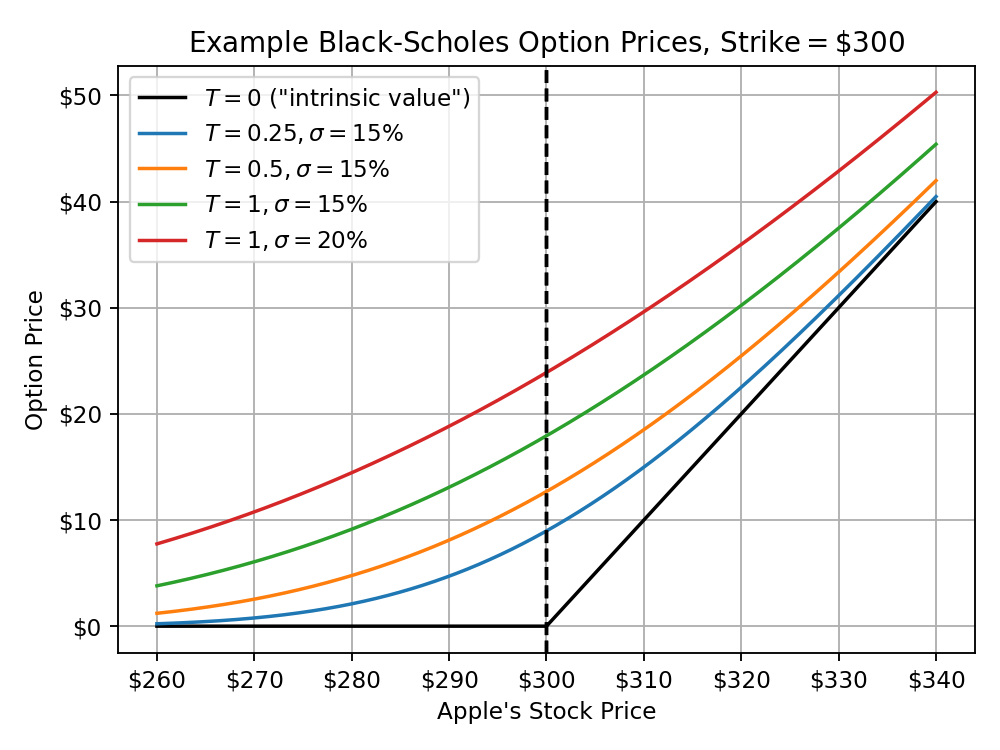
If your option is expiring in \(T\) years, we already know $$ \begin{aligned} S(T) &\sim S(0) \cdot \exp\left[N\left(-\frac{\sigma^2}{2} \cdot T, \sigma^2\cdot T\right)\right]\\ &\sim \exp\left[N\left(\ln S(0) - \frac{\sigma^2}{2} \cdot T, \sigma^2\cdot T\right)\right] \end{aligned} $$

One such distribution is shown below, with the portion above the strike shaded in blue. That’s where we need to take the average!

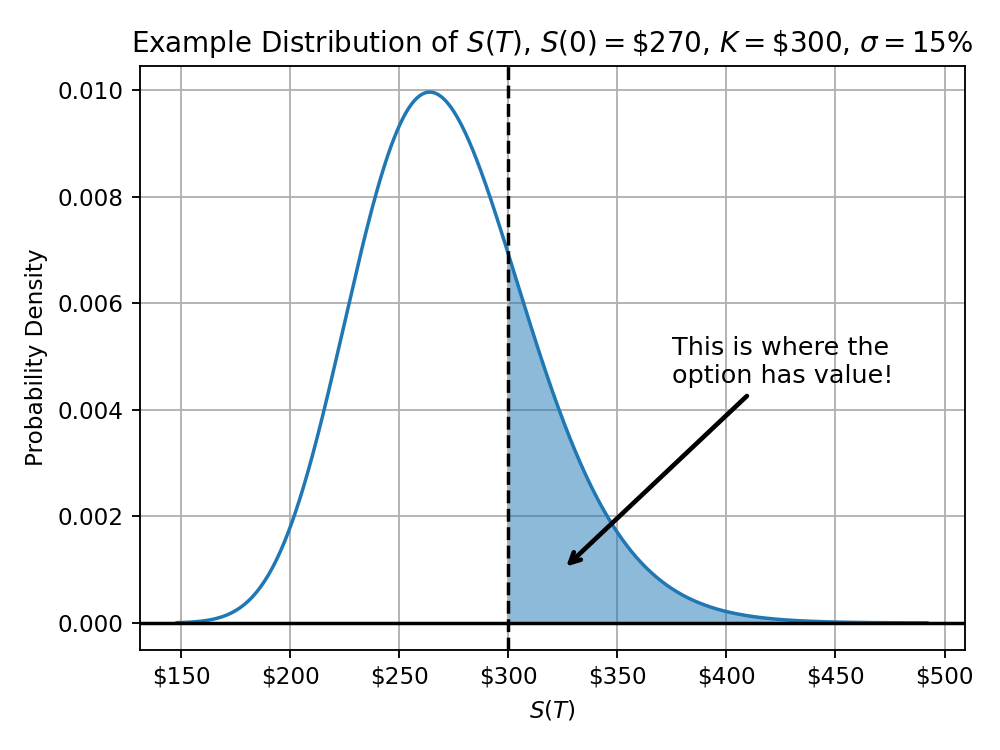
So, let’s denote the price of our (call) option as \(\widetilde{C}\). We decided that this should equal the average profit of the option. $$ \begin{aligned} \widetilde{C} &= \mathbb{E}\left[S(T)-K \mid S(T) > K\right]\\ &= \mathbb{E}\left[S(T) \mid S(T) > K\right] - K \cdot \mathbb{P}\left[S(T) > K\right] \end{aligned} $$

Computing the probability term

#

Looking at the second term, note that $$ \begin{aligned} K \cdot \mathbb{P}\left[S(T) > K\right] &= K \cdot \mathbb{P}\left[\ln\left(\frac{S(T)}{S(0)}\right) > \ln\left(\frac{K}{S(0)}\right)\right]\\ &= K \cdot \mathbb{P}\left[N\left(-\frac{\sigma^2}{2} \cdot T, \sigma^2\cdot T\right) > \ln\left(\frac{K}{S(0)}\right)\right]\\ &= K \left[1-\Phi\left(\frac{\ln\left(\frac{K}{S(0)}\right) + \frac{\sigma^2}{2} \cdot T}{\sigma \cdot \sqrt{T}}\right)\right] \end{aligned} $$ where the last step comes from rescaling everything to a standard normal distribution.

Computing the expectation term

#

Now, let’s figure out the average stock price for that expectation term. Luckily, we’ve already done this integral!⁵ $$ \begin{aligned} \mathbb{E}\left[S(T) \mid S(T) > K\right] &= \int_K^{\infty} x \cdot f_{S(T)}(x) \text{ d}x\\ &= \int_K^{\infty} x \cdot f_{\exp\left[N\left(\ln S(0)-\frac{\sigma^2}{2} \cdot T, \sigma^2 \cdot T\right)\right]}(x) \text{ d}x\\ &= S(0) \cdot \left[1-\Phi\left(\frac{\ln\left(\frac{K}{S(0)}\right) - \frac{\sigma^2}{2}\cdot T}{\sigma \sqrt{T}}\right)\right] \end{aligned} $$

Finishing the derivation

#

Bringing the terms together, we see $$ \begin{aligned} \widetilde{C} &= S(0) \cdot \left[1-\Phi\left(\frac{\ln\left(\frac{K}{S(0)}\right) - \frac{\sigma^2}{2}\cdot T}{\sigma \sqrt{T}}\right)\right] - K \left[1-\Phi\left(\frac{\ln\left(\frac{K}{S(0)}\right) + \frac{\sigma^2}{2} \cdot T}{\sigma \cdot \sqrt{T}}\right)\right]\\ &= S(0) \cdot \Phi\left(-\frac{\ln\left(\frac{K}{S(0)}\right) - \frac{\sigma^2}{2}\cdot T}{\sigma \sqrt{T}}\right) - K \cdot \Phi\left(-\frac{\ln\left(\frac{K}{S(0)}\right) + \frac{\sigma^2}{2} \cdot T}{\sigma \cdot \sqrt{T}}\right)\\ &= S(0) \cdot \Phi\left(\frac{\ln\left(\frac{S(0)}{K}\right) + \frac{\sigma^2}{2}\cdot T}{\sigma \sqrt{T}}\right) - K \cdot \Phi\left(\frac{\ln\left(\frac{S(0)}{K}\right) - \frac{\sigma^2}{2} \cdot T}{\sigma \cdot \sqrt{T}}\right) \end{aligned} $$

And that’s the Black-Scholes formula! This is more commonly simplified into $$ \widetilde{C} = S(0) \cdot \Phi\left(d_+\right) - K \cdot \Phi\left(d_-\right) $$ with $$ d_+ = \frac{\ln\left(\frac{S(0)}{K}\right) + \frac{\sigma^2}{2}\cdot T}{\sigma \sqrt{T}},\quad d_- = d_+ - \sigma\sqrt{T} $$

One final financial consideration

#

There’s one extra detail I’ve glossed over – money today is “worth more” than money in the future.

In the Black-Scholes world, this is simply encoded as a “risk-free rate” \(r\) where cash grows exponentially in value over time. $$ \text{Cash}(t) = e^{rt} \cdot \text{Cash}(0), \quad \text{Cash}(0) = e^{-rt} \cdot \text{Cash}(t) $$

Accounting for this just requires

1. Converting our current price \(S(0)\) to future value \(\left[e^{rT} \cdot S(0)\right]\), and
2. Converting the future option price \(\widetilde{C}\) to current value \( \left[e^{-rT} \cdot \widetilde{C}\right]\)

Simplifying with \(D = e^{-rT}\) gives us the actual Black-Scholes formula. $$ C = D \left[\frac{S(0)}{D} \cdot \Phi\left(d_+\right) - K \cdot \Phi\left(d_-\right)\right] $$

See also and references

#

For some more background on options and the Black-Scholes pricing model, consider the following Wikipedia pages.

• Option and Option style, which discusses some common variants of options other than the “European call options” considered here
• Put-call parity, which lets you derive “put option” prices once you have a model for call option prices
• Geometric Brownian Motion, the stochastic diffusion process assumed in this model for the stock price \(S(t)\)
• Black-Scholes model and Black-Scholes equation (particularly the “Derivation” section for the more traditional approach)
• Itô’s lemma, the stochastic calculus version of the chain rule that’s used in traditional Black-Scholes derivations
• Rational option pricing via delta hedging and Delta neutral for the hedging strategy used in the traditional derivation