A few months ago, I was personally interested in using a back-of-the-envelope estimate to try to quantify the impact a stale calibration has on the performance of a tail risk model.
Here, I’ll provide some context for this question and a simple experiment I ran to explore it.
Background #
Tail risk models #
A relatively common task in finance is to forecast confidence intervals for future prices for a particular product or asset. This is particularly important for gauging how much risk you are taking on in that asset.
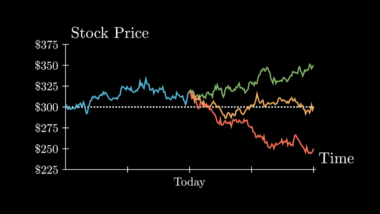
For example, if I’ve seen the historical behavior of a stock price, what is my best guess on how that price may evolve in the next week? The next month?
![Nvidia's historical stock price drifts down from $140 to $100 over 6 months. The future projection for a 95%
profile and 5% profile start close together, but expand to [$80, $200] over the next 3 months.](/stale-calibration-backtest/example-t-levy-process-profiles.webp)
Notably, the purpose of such a model depends on your use case.
If I own this stock, I’m predominantly concerned about the price decreasing. This is “market risk”.
If I’ve agreed to pay someone a fixed amount in exchange for their stock in the future, I’m additionally concerned about the price increasing.
That’s the money at risk in a counterparty default scenario. It should represent a profit for me, but I would lose it if the other party fails to uphold their end of the deal. This is “counterparty risk”.1
More generally, I’d refer to this as “tail risk”, so-called because the risk corresponds to low-probability events from the tail of a statistical distribution.2
Calibrating a model #
Any tail risk model fundamentally relies on assumptions about how the product’s price will evolve over time.
Usually, this involves a set of parameters (e.g., a stock’s volatility and expected drift) that are fit to historical data or the market’s current expectations. The fitting process is referred to as “calibration”.
Importantly, this should be re-evaluated periodically. Ideally, quite frequently! Recent data is a better indication of the future than older, “stale” data.
The main question is: how long should we go before we recalibrate? This becomes especially important if
- The model is extremely expensive or difficult to recalibrate,
- The data required to recalibrate is unavailable or infrequently available,
- Calibrations have to align with technology release schedules,
- Calibrations are temporarily impossible due to system issues, technology freezes, and so on.
Example tail risk model #
For the purposes of this experiment, I’m taking a somewhat simple model of stock prices and am interested in two-week price changes as a typical margin period of risk.
\(t\)-distribution Levy process #
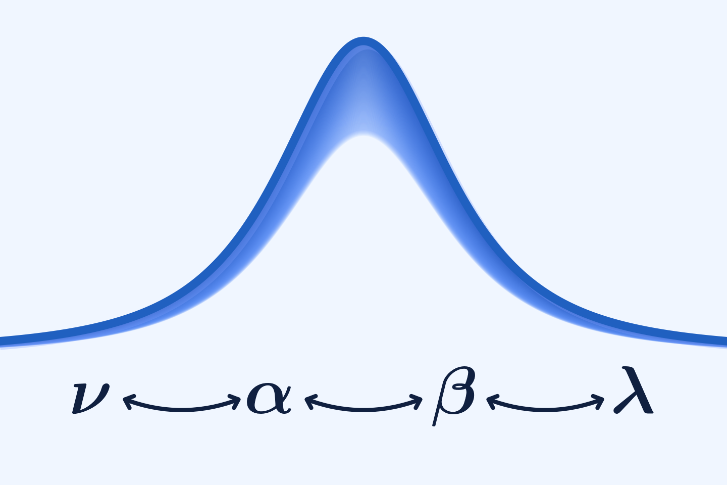
Take daily log-returns of the stock as drawn from a \(t\) distribution, \(\Delta (\log S_t) \sim t(\mu, \sigma, \nu)\). Then,
- \(\mu\) determines the drift of the stock price,
- \(\sigma\) determines its volatility, and
- \(\nu\) determines how fat the tails are.
You can think of this as Geometric Brownian motion but with fatter tails so that extreme events are more likely than a normal distribution would imply.
Afterward, we can simulate draws from the distribution and forecast possible changes in the stock price step-by-step.3
Naively, we can calibrate such a model by simply fitting a \(t\) distribution to historical returns. Below, I choose a 3-year calibration window as a reasonable middle ground between using recent history and having sufficient data length.
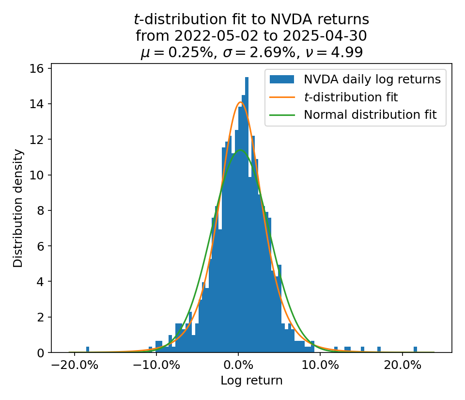
The calibration fit has given us estimated values for the three parameters \(\mu, \sigma, \nu\), which we could use in our future forecasts.
However, as shown here, this is essentially a maximum likelihood fit with all data equally weighted, which is not ideal.
Calibration by exponentially decaying flexible probabilities #
Remember, earlier we mentioned that “recent data is a better indication of the future”!
We can incorporate this idea into the calibration itself by weighting the more recent historical data more than older data. A standard way to do this is with exponentially decaying weights, $$ p_t = \frac{\exp\left(-\dfrac{\ln 2}{\tau_{HL}} \lvert\bar{t} - t\rvert\right)}{\sum_s p_s} $$ where \(\tau_{HL}\) is the half-life describing how quickly the weights get cut in half, and the denominator normalizes the weights to sum to 1.
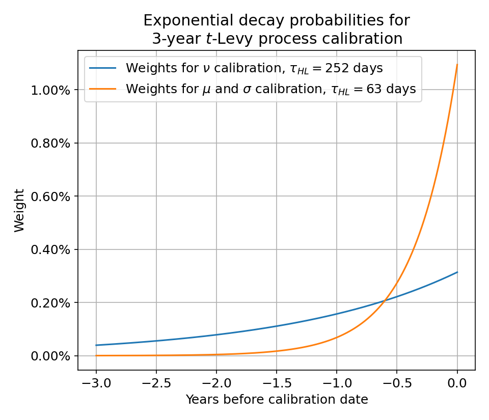
If we use the above weights, our calibration will automatically4 “prioritize” recent behavior.
Importantly, I’m using a much longer half-life (1 year) for the calibration of the tailedness \(\nu\) than for the drift \(\mu\) and volatility \(\sigma\) (1 quarter). It is simply much harder to determine the degree to which data is fat-tailed, so you tend to need more data for a reliable estimate.
In general, this is a tradeoff between how responsive you want the model to be and how stable you want the parameters (and therefore your risk forecasts) to be. In my case, I found the above choices to have good empirical coverage (the 5% and 95% profiles were reasonably accurate) and relatively stable parameters.
Stability of parameter estimates #
Below, I plot the calibration parameters we get for Eli Lilly (LLY) as our calibration cutoff date varies.
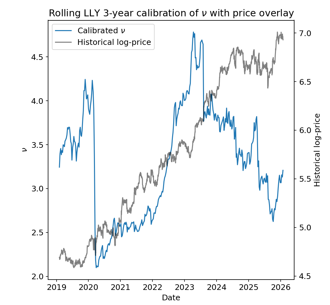
Here, \(\nu\) is quite stable, and most years have its value hovering within a band of width ~0.5.
The most notable exception is the rapid drop from ~4.0 to ~2.5 immediately following the COVID crash of March 2020. This was an incredibly extreme market event compared to the rest of the recent history, so the calibration responded by making the tails significantly fatter (smaller \(\nu\)).
In fact, this rapid reaction to an extreme market event is a feature of the exponentially weighted calibration!
On the other hand, one could argue that its effect should diminish more rapidly over the following years. In our case, \(\nu\) does not fully recover to pre-COVID levels until 2023 when the 3-year calibration window no longer includes the crash at all.
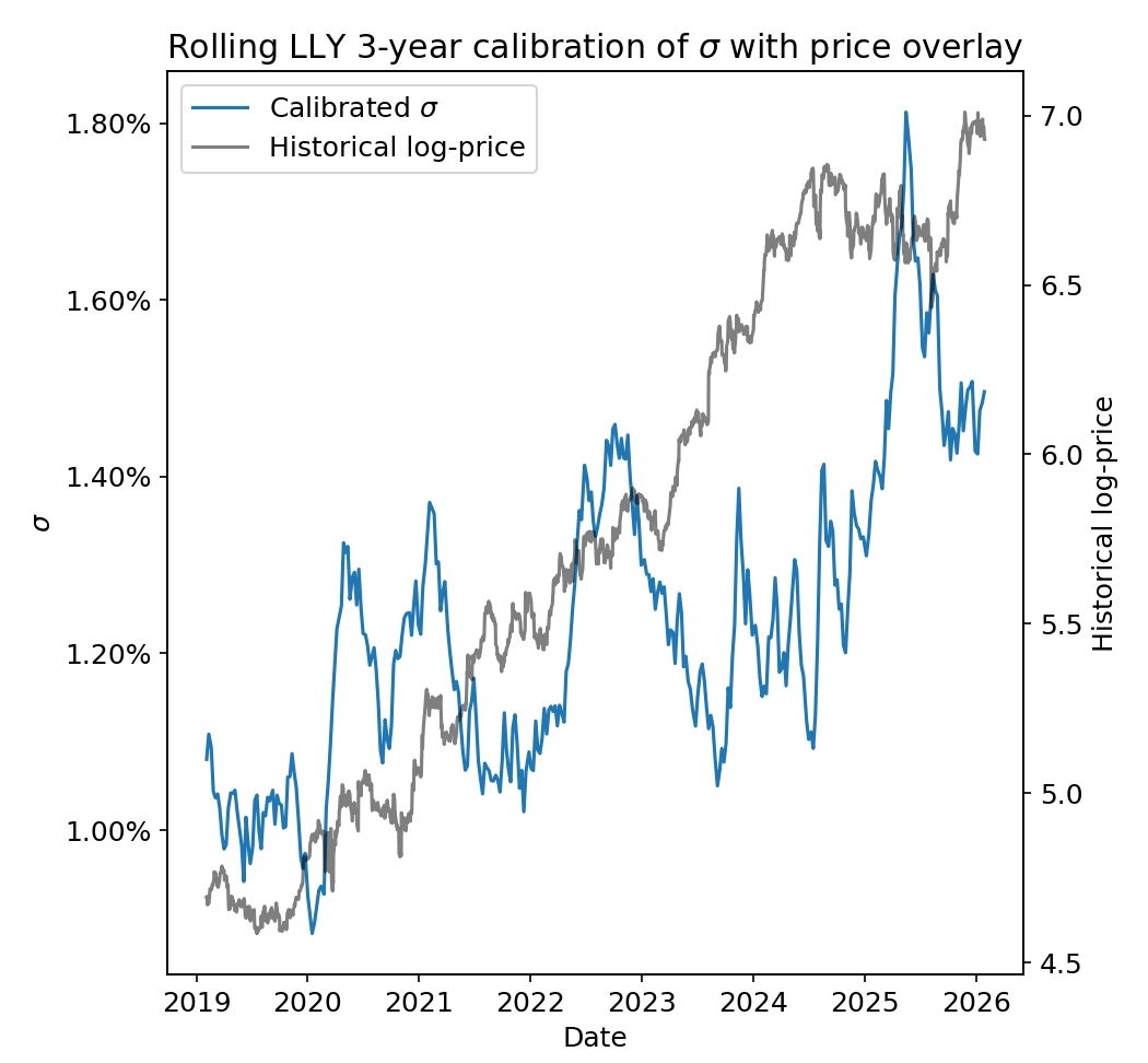
The calibration for \(\sigma\) is slightly more volatile but still reasonably stable overall. This parameter will tend to be more reactive than \(\nu\) due to the significantly shorter half-life of 1 quarter in the calibration weights.
Notably, the COVID crash does not have an enormous impact on the volatility! The COVID shock is largely absorbed by the changes in \(\nu\) by making the tails fatter.
Indeed, a decreasing \(\nu\) (fatter tails) “looks like” an increasing volatility \(\sigma\)! These are complementary effects that capture different aspects of the severity vs. frequency of large price movements.
Basic backtesting #
As noted earlier, our model’s purpose is to generate a one-tailed 95% confidence interval for how much the stock price may increase (for counterparty risk calculations).
As such, if new stock price data exceeds our confidence interval significantly more than 5% of the time, our model is doing a bad job. The simplest way to formalize this is through a Binomial test.
Let’s say we’re judging our model’s prediction of 2-week returns with one year of new data.
- We have \(n = 25\) samples of 2-week returns, and
- We observe \(k\) breaches (exceedances) of our confidence interval. Then,
- Our Binomial test’s \(p\)-value is \(p = P(X \geq k)\) where \(X \sim B(n, p=5\%)\).
If you chose a significance level of \(\alpha = 1\%\) for the test, we have the following possible results:
| Breaches (exceedances) | Binomial test \(p\)-value | Result |
|---|---|---|
| 0 | 100.0% | PASS |
| 1 | 72.3% | PASS |
| 2 | 35.8% | PASS |
| 3 | 12.7% | PASS |
| 4 | 3.4% | PASS |
| 5 | 0.7% | FAIL |
Real backtesting calculations can be significantly more complicated, but importantly, this style of calculation is often treated as a de facto judge of whether the model is working properly.
In other words, the \(p\)-value (or an equivalent calculation) becomes a performance metric of its own, either for simplicity or imposed in regulatory requirements. Teams may discuss or compare models directly in terms of their backtesting \(p\)-values as proof that the model is performing well (or not)!
So, it would be nice if we could talk about the “impact” of a stale calibration in the same terms. “What impact does a stale calibration have on our backtesting metric?”
Backtesting impact of a stale calibration #
Something we can try is to “backtest the model against itself”, one version with stale calibration parameters and another with newer parameters.
The idea here is to create a clean, ideal comparison that focuses only on the calibration impact and ignores all model insufficiencies and difficulties of real market data.
To be specific, we take two calibrations of the same model:
- One new (freshly) calibrated version that we will draw simulated data from.
- One stale version with outdated calibration parameters that we will use to forecast tail risk in the backtest.
Over many trials, we can generate a distribution of backtesting \(p\)-values and judge how much more frequently the stale model is failing compared to the intended significance level, \(\alpha\).
Again, this is effectively assuming your model form is perfect so that we are backtesting only the changes in calibration parameters.
Historical stress example #
To judge how bad a stale calibration could get, we can take a particularly bad historical crash as an example.
In this case, we draw historical data from an AAPL model whose calibration includes the COVID crash in March 2020 and backtest an AAPL model that has never seen this crash.
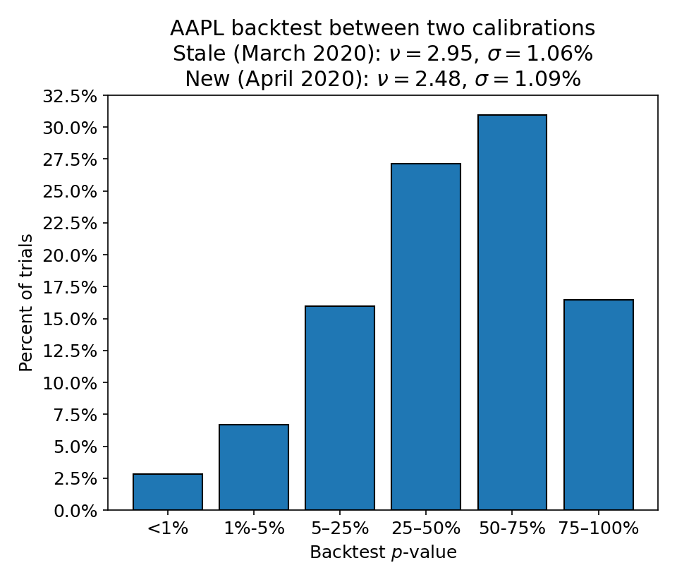
Here, we can see that ~2.5% of the \(p\) values are below 1% and about ~10% are below 5%. In this sense, the model is performing about 2.5x worse than it would if the model were always recalibrated immediately.
It’s important to remember that we are treating the newly calibrated model as ground truth! This is not a direct reflection of the market data of this period but rather the speed at which the model’s calibration would have updated if it were refreshed more frequently.
This means that the impact of the stale calibration is effectively a shift in the failure threshold of our backtest. It is as though we’ve shifted our \(\alpha = 1\%\) to \(\alpha = 2.5\%\).
Extrapolations of parameter drift over time #
Rather than picking a particular stress scenario, we would prefer to be able to estimate how quickly the model performance would degrade over time.
Realistically, you would not spend much time modeling the behavior of the calibration parameters. If you’re trying to improve a model, you’d better spend that effort on the model itself! But we can still calculate rough estimates from historical trends.
Below, I’ve taken the average drift speed of each calibration parameter from historical calibrations and extrapolated those trends out to gauge the degradation of backtesting performance as the calibration gets more and more stale.
This is quite a conservative estimate as I am taking several simplifying assumptions.
- All parameters are trending in a direction that makes your risk estimate worse: fatter tails (smaller \(\nu\)), higher drift (larger \(\mu\)), and higher volatility (larger \(\sigma\)).
- The changes in each calibration parameter are independent so that they can each drift according to average historical speeds.
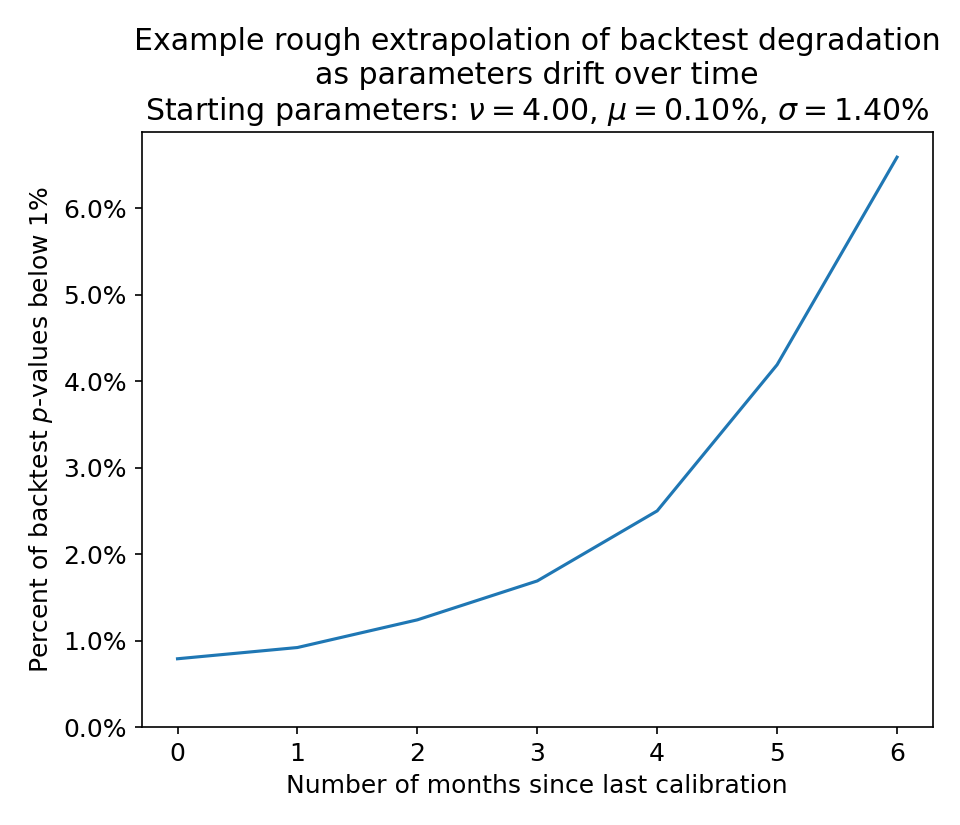
All caveats aside, we can see there is very little impact to backtesting performance with 1-2 months of stale calibration. The backtest still fails around 1% of the time, as expected.
The performance degrades a bit more to failing around 2% of the time with 3-4 months of staleness, with significantly worse results afterward.
In other words, it is probably acceptable to calibrate the model quarterly (every 3 months), but less frequently would likely result in unacceptable performance.
Final thoughts #
In general, I think it is useful to tie model insufficiencies or limitations directly to the concerns of your stakeholders / management teams.
Here, we’ve been tying the discussion to a performance metric used to judge the quality of the model.
For example, we could (roughly) estimate that if we were forced to hold off on calibrations for 3 months, the model may fail backtesting twice as often as expected from the statistical test. This would be quite useful in discussions with teams concerned about the model performance metric itself.
However, saying “the model would be twice as bad in backtesting”
- Doesn’t give a sense of “how bad is acceptable”, even if you only care about the backtesting \(p\)-value.
- Doesn’t quite mean much about the true use of the model. We’re estimating tail risk! How far off are we?
The whole point of this thought experiment was to directly tie stale calibrations to a model performance metric, but there are other angles that would be more appropriate for other stakeholders.
- How much would we be underestimating tail risk? On a relative basis? In absolute dollar terms?
- How frequently would we miss risk that should be breaching limits?
- How much trading activity would we be allowing that should have been pre-emptively halted?
In such cases, the analysis would need to be tweaked accordingly. Luckily, the above questions are typically a bit easier to estimate.
See also and references #
This discussion was intended to be relatively comprehensive and self-contained, but feel free to reference some of the general resources below for more information.
There is also an informal ~10-minute version of this discussion available on YouTube and the code for this analysis is on GitHub.
- The Wikipedia pages on tail risk, model calibration, geometric Brownian motion, Levy process, and Monte Carlo simulations.
- The Value-at-Risk (VaR) backtesting discussions of Investopedia, MATLAB, and AnalystPrep. These resources discuss more sophisticated statistical tests and many difficulties or shortcomings that I have intentionally omitted here.
- The Basel Committe’s “Sound practices for backtesting counterparty credit risk models” from December 2010 that provides significantly more guidance on how to properly backtest financial models.
Typically, there are legal agreements in place that force the other party to uphold their end of the deal. In that case, this becomes “counterparty credit risk” where the other party may go bankrupt before the deal is finalized. ↩︎
I see that Wikipedia and Investopedia use a stricter definition that focuses on percentiles \({\leq} 0.3\%\) and \({\geq} 99.7\%\), but I have never personally seen this cause confusion. ↩︎
Here, I’m using a simulation for simplicity, but in this case, we could actually compute the forecast confidence intervals directly with a Fourier transform. However, simulations are generally required for more sophisticated models. ↩︎
Actually, I’m now performing the calibration in two steps since the reweighting from \(\nu\) to \((\mu,\sigma)\) fundamentally changes the data set that we’re calibrating to.
You probably could use a fancier optimization technique that takes the per-parameter weights into account, but my intuition is that this would come at the cost of worse parameter stability over time. ↩︎